

DNA is a complex molecule that contains instructions for life and often referred to as a “digital fingerprint” or code telling a cell what to do. DNA is often the only means for accurate testing and identification of biomolecules, cells, or even an entire person during forensic investigations. The need to be able to test for DNA, as quickly as possible, and even at the site where the sample is taken, is becoming more and more important.
Polymerase Chain Reaction (PCR) and DNA Amplification
The more DNA one has in a sample, the easier it is to identify and diagnose. In many situations, such as old crime scenes or large ecological systems with dilute samples, you want to amplify the amount of available DNA before testing for it. One technique that is most effective in amplifying DNA and making it useful in medical diagnostic, chemical, and biological analysis is Polymerase Chain Reaction, commonly known as PCR. It is also referred as a DNA amplification technique. Further, there has been great interest in recent years in developing portable PCR-based micro total analysis systems (μTAS; also known as lab-on-a-chip systems) for point-of-care applications.
One strategy that seems very promising is natural convection-based PCR. In this strategy, many copies of a DNA template can be made by cycling between hot and cold regions within a microreactor via a buoyancy-driven flow. The multiphysics nature of this strategy makes it a perfect candidate for simulations with COMSOL software.
A COMSOL model can provide more quantitative understanding of the dynamics and kinetics involved in the process that will be very useful in designing and developing efficient μTAS. Here, I will show you a model that was developed to study the spatio-temporal variation of the concentrations of single-stranded (ssDNA), double-stranded (dsDNA), and primer-annealed (aDNA) DNA components during natural convection-based PCR. The model is available for download from the Model Gallery.
The driving mechanism for the fluid motion is the temperature-induced density differences that results in buoyancy flow. This approach eliminates the need for an external driving mechanism as the difference between the temperatures is sufficient to circulate the PCR mixture and amplify DNA in a closed loop, as shown below.
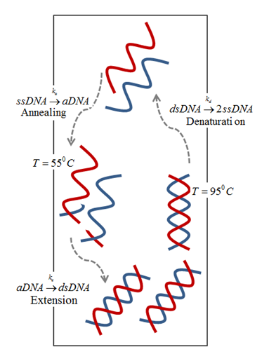
Schematic of buoyancy-driven PCR.
In general, a PCR mixture consists of a DNA template, primers, nucleotides, and the enzymes (Taq polymerase, the most widely used amplifying enzyme). The mixture is repeatedly cycled between three temperature zones:
- Denaturing zone (95°C): Double-stranded DNA template is separated into two single strands.
- Annealing zone (55°C): Primers bind to the ends of the single-stranded DNA.
- Extension zone (72°C): A complement to each of the annealed single strands is created by enzyme resulting in two new copies of double strands DNA template. Repeating the above process results in an exponential increase in DNA concentration.
Developing a Bouyancy-Driven PCR Model
In the figure above, you can see the 2D model geometry of the buoyancy-driven PCR. A dilute PCR mixture fills the channel with an impermeable wall. The right and left boundaries of the channel are maintained at 95°C and 55°C, respectively. The upper and lower boundaries are insulated. The temperature gradient produces variation in the density of fluid that drives the buoyant flow. The model uses temperature-dependent properties for water. The predefined Non-Isothermal Flow/Conjugate Heat Transfer interface available in the CFD Module or the Heat Transfer Module is used to model coupled heat transfer and the fluid flow physics.
The DNA components are generated and consumed by the temperature-dependent chemical reactions as proposed in “Polymerase chain reaction in natural convection systems: A convection–reaction-diffusion model” by E. Yariv, G. Ben-Dov, and K. D. Dorfman. A simplified first-order reaction mechanism (given below) illustrates the PCR process that is used in this model. The rates of change in the concentration of DNA components were determined from the stoichiometric balances.
\mathit{dsDNA}\xrightarrow{k_d}2\mathit{ssDNA} Denaturation (95°C)
\mathit{ssDNA}\xrightarrow{k_a}\mathit{aDNA} Annealing (55°C)
\mathit{aDNA}\xrightarrow{k_e}\mathit{dsDNA} Extension (72°C)
These reaction rates constants were spatially modulated using the below Gaussian mapping function. This is done in order to localize each reaction in its respective temperature zone.
Here, \sigma (=1°C) is the standard deviation of the reaction rate with respect to temperature and T_i is the ideal temperature for denaturation (95°C), annealing (55°C), and extension (72°C) reaction (at which the function is maximized). The multicomponent mass transfer of DNA components in the channel is governed by the convection and diffusion equation, and is modeled using the Transport of Dilute Species interface from the Chemical Reaction Engineering Module.
A step-wise approach is used to solve the coupled system of heat transfer, fluid flow, and mass transfer. Non-Isothermal Flow physics is solved at steady state, and the velocity field that is obtained is used in the mass transfer equation to obtain time varying concentrations of DNA components.
Modeling Results
Below, we can see the steady-state velocity profile and temperature contours across the channel. We can note that a large convective cell occupies the channel and the fluid flows along the boundaries and is faster at the vertical walls where the temperature variations are highest.
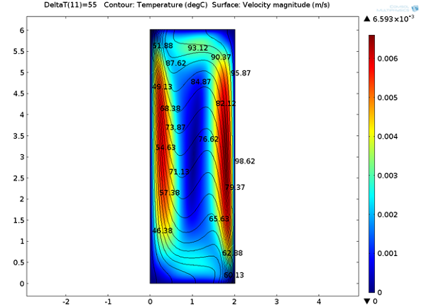
Temperature distribution and velocity magnitude.
Next, we can look at the reaction rates for denaturation, annealing, and extension reactions after 120 seconds. It is clear that these reactions are localized around 95°C, 55°C, and 72°C respectively. It will be interesting to see the variation of these reaction rates with respect to time.
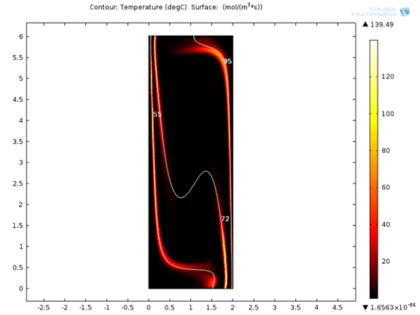
Reaction rates for denaturation, annealing, and extension reactions after 120 s.
Initially only denaturation is taking place in the channel, but after a certain amount of time, annealing and extension effects are also visible.
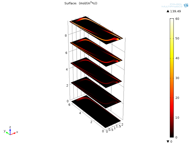
Variation of reaction rates for denaturation, annealing, and extension with time.
Interesting results are obtained when the concentrations of DNA components are monitored. In the plot below, you can see the concentration profile of DNA components for a simulation time of 120s.
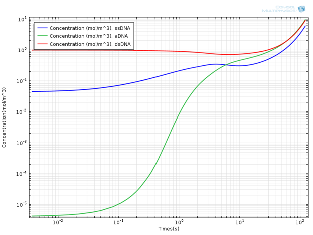
Concentration Profile of DNA Components.
It is evident that the concentration of the double-strand DNA template (dsDNA) initially decreases due to denaturation, but later on exponentially increases due to the amplification effect in the extension region. It is common to use the doubling time in order to quantitatively characterize PCR efficiency. The doubling time is the time required to double the concentration of initial double-strand DNA template (dsDNA) used in the mixture. From the concentration plot, the doubling time is around 60 seconds, which is of the same order of magnitude as given in the aforementioned literature. In general, the doubling time of a laboratory scale conventional PCR system is around two minutes.
Conclusion and Next Steps
This blog post briefly described a multiphysics model for DNA amplification by PCR in a buoyancy-driven flow. It can be used to understand the amplification rates as a function of the device parameters, which will be very useful in device design and optimization. More realistic reaction data can be brought on-board, and geometric parameters can be varied. In general, it is possible to extend the scope of this model using the powerful and flexible user interfaces of the Heat Transfer, CFD, and Chemical Reaction Engineering modules.

Comments (0)