Nonlinear Structural Materials Module

Expand Structural Analyses with a Variety of Nonlinear Material Models

Many materials have a nonlinear stress–strain relationship, particularly at higher stress and strain levels. When analyzing objects made of such materials, you need to account for these nonlinearities. The Nonlinear Structural Materials Module, an add-on to either the Structural Mechanics Module or MEMS Module, contains dozens of material models to help you model a wide range of solid materials.

The Geomechanics Module, a similar but separate add-on to the Structural Mechanics Module, is specifically developed for materials common in geotechnical applications such as soils and rocks.

Contact COMSOL
A silver stent model showing the stress in blue at maximum expansion.
 

Nonlinear Structural Materials for Multiphysics Modeling

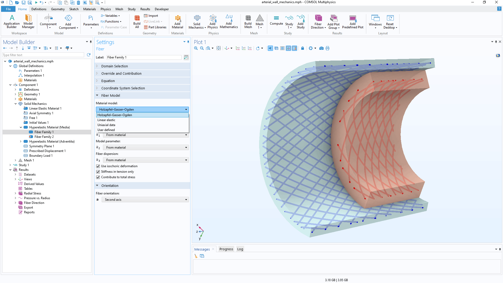
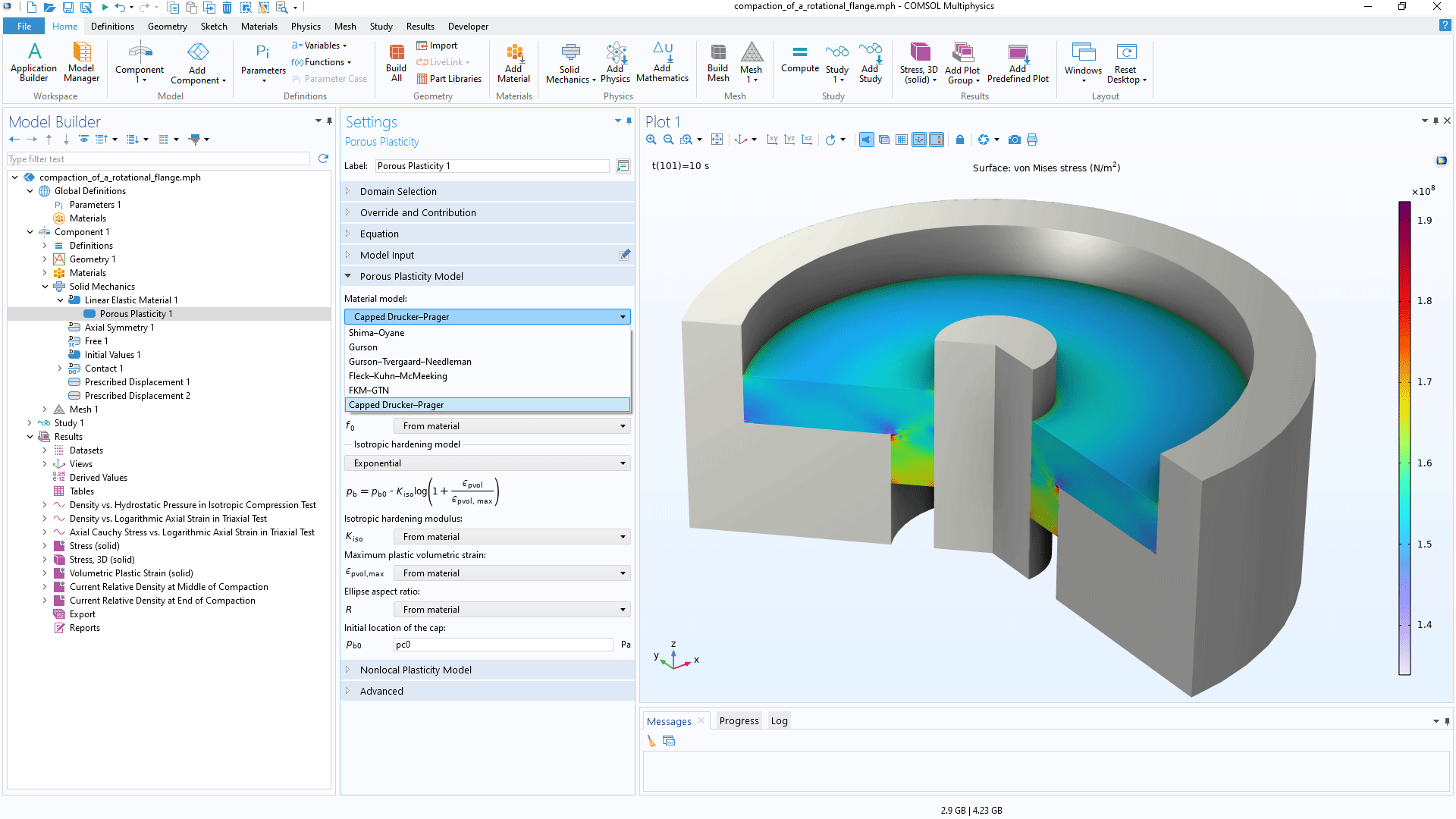
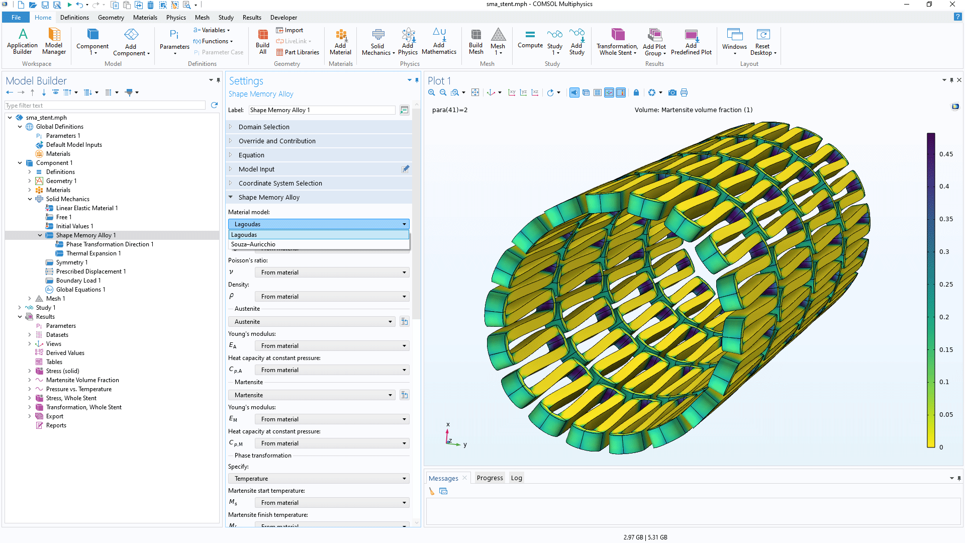
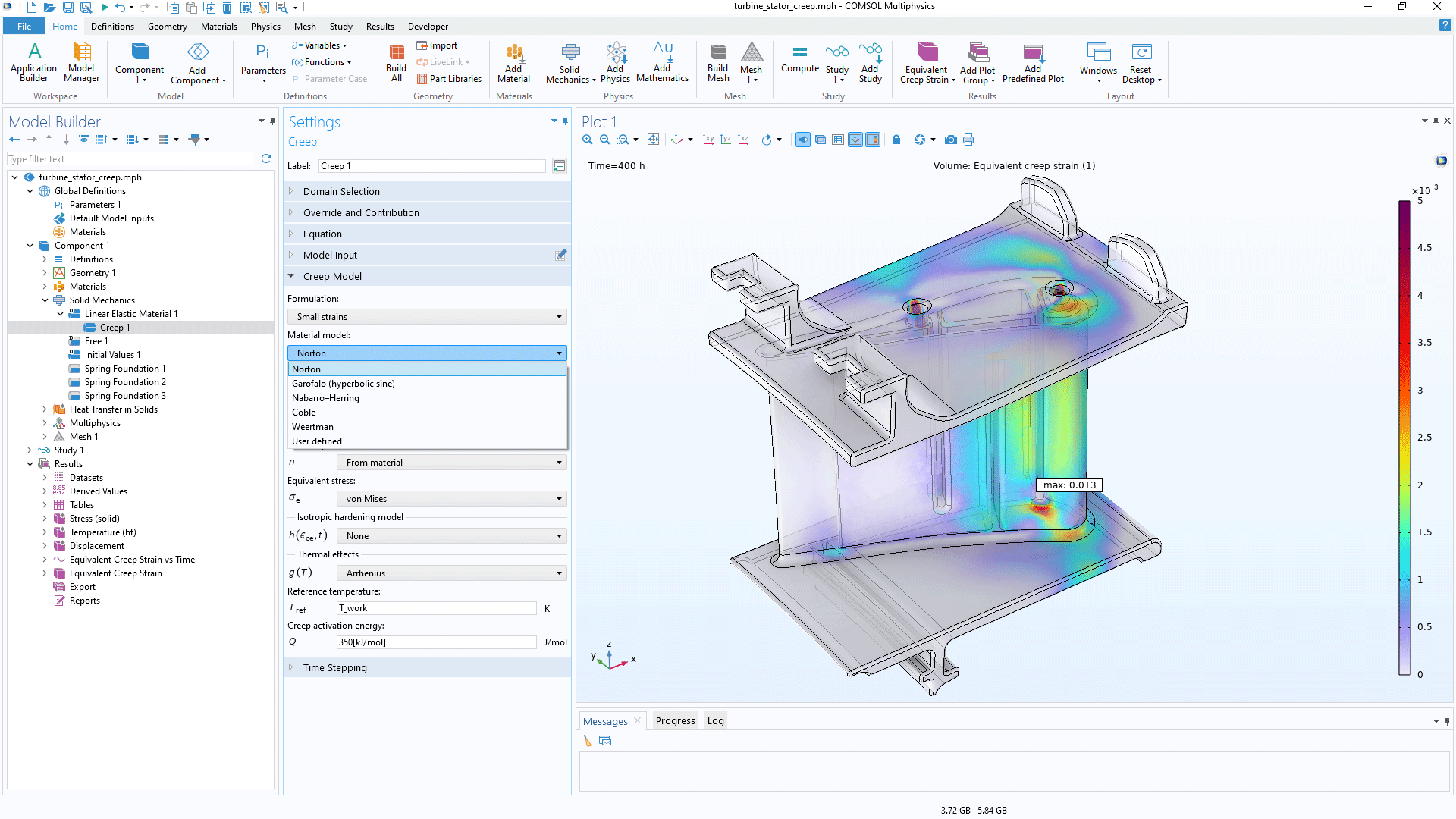
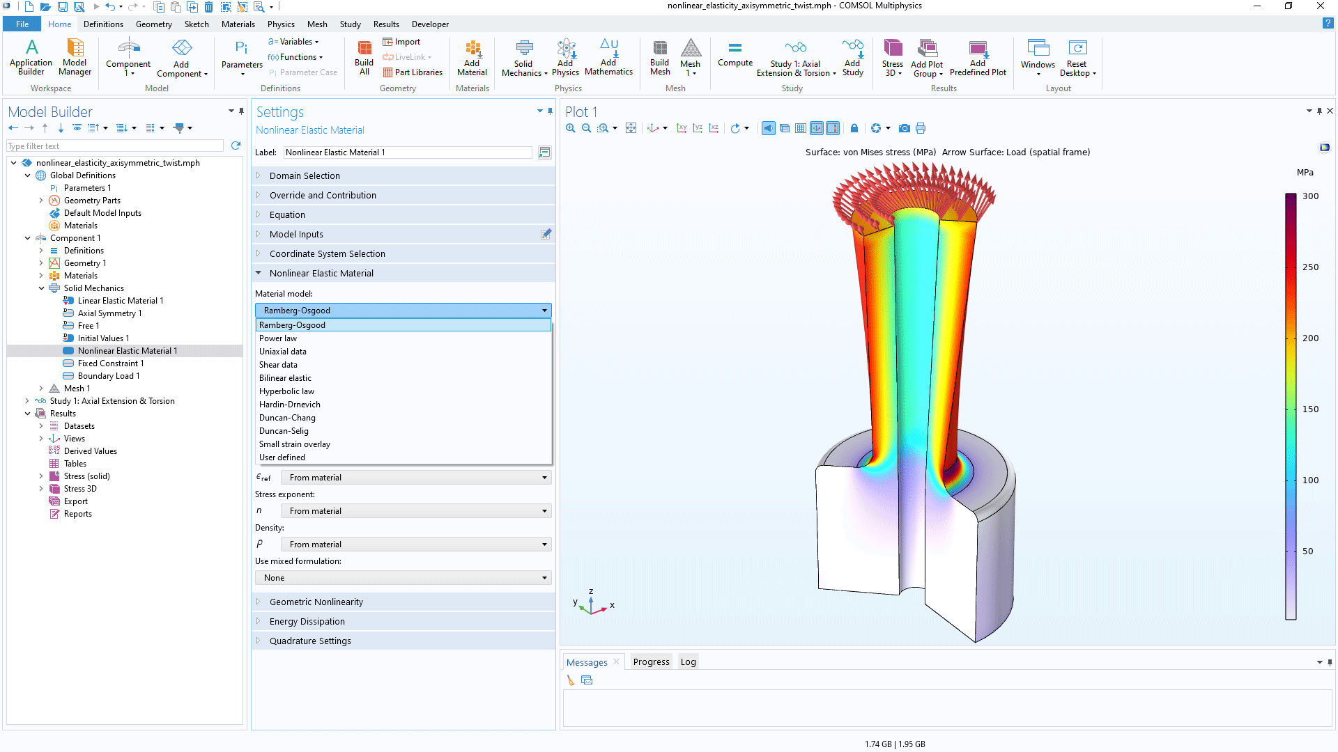
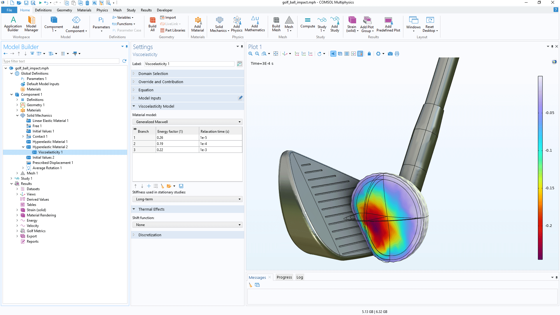
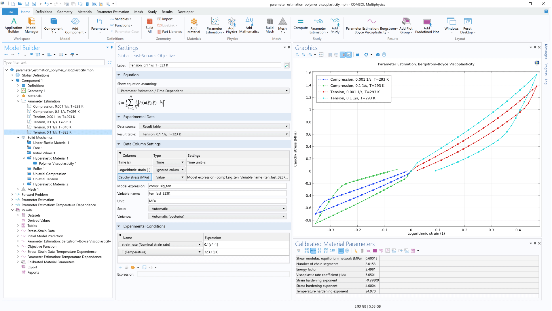
The functionality for modeling nonlinear materials augments all of the structural analyses available within the Structural Mechanics Module or the MEMS Module. Combine linear elastic, hyperelastic, or nonlinear elastic materials with nonlinear effects such as plasticity, creep, viscoplasticity, or damage, and use the versatility of the COMSOL Multiphysics® simulation software to include multiphysics couplings with a couple of clicks. You can even define your own models based on, for example, stress or strain invariants. Create your own flow rules and creep laws, as well as your own strain energy density functions for hyperelasticity.

Multiphysics capabilities are built into the COMSOL Multiphysics® software platform for modeling thermal expansion, pore pressure, fluid–structure interaction, and many more multiphysics phenomena. All of the structural materials included in the Nonlinear Materials Module are multiphysics capable.

Material Models in the Nonlinear Structural Materials Module

The numerous material models available are listed below, with screenshots of their implementation in the software.

A close-up view of the Fiber settings and an arterial wall model in the Graphics window.

Hyperelasticity

Hyperelastic constitutive laws are used to model materials with a nonlinear relation between stress and strain based on a strain energy density function. This type of material is typically found in rubber, foam, and biological tissue. Many different hyperelastic material models are available in the Nonlinear Structural Materials Module, but you can also define your own strain energy density functions. The following hyperelastic models are available:

  • Arruda–Boyce
  • Blatz–Ko
  • Delfino
  • Extended tube
  • Fung anisotropic
  • Gao
  • Gent
  • Mooney–Rivlin
    • Two parameters
    • Five parameters
    • Nine parameters
  • Murnaghan
  • Neo–Hookean
  • Ogden
  • St. Venant–Kirchhoff
  • Storakers
  • van der Waals
  • Varga
  • Yeoh
  • Fibers (anisotropic hyperelasticity)
    • Holzapfel–Gasser–Ogden
    • Linear elastic
    • Uniaxial data
    • User-defined anisotropic hyperelasticity
    • Thermal expansion in fibers
  • Mullins effect
    • Ogden–Roxburgh
    • Miehe
  • Large-strain
    • Viscoelasticity
    • Viscoplasticity
    • Creep
    • Polymer viscoplasticity
  • Phase-field damage
A close-up view of the Porous Plasticity settings and a powder compactor model in the Graphics window.

Porous Plasticity

The modeling of plastic deformation in soils, porous metals, and aggregates has a main difference with respect to traditional metal plasticity: the yield function and plastic potential are not only defined in terms of the deviatoric stress tensor, but also include dependencies on the hydrostatic pressure. The following porous plasticity models are available:

  • Shima–Oyane
  • Gurson
  • Gurson–Tvergaard–Needleman
  • Fleck–Kuhn–McMeeking
  • FKM–GTN
  • Capped Drucker–Prager
  • Large-strain porous plasticity
  • Nonlocal plasticity
    • Implicit gradient
A close-up view of the Shape Memory Alloy settings and a stent model in the Graphics window.

Shape Memory Alloys

Shape memory alloys refer to materials that can remember their original shape after undergoing large deformations, when heated above a certain temperature. The material models available in the Nonlinear Structural Materials Module provide the necessary settings for the austenite and martensite start and finish temperatures, as well as important phase transformation parameters. Two common SMA models are available: Lagoudas and Souza–Auricchio.

A close-up view of the Creep settings and a turbine stator model in the Graphics window.

Creep and Viscoplasticity

Creep is an inelastic time-dependent deformation that occurs when a material is subjected to stress (typically much less than the yield stress) at sufficiently high temperatures. In COMSOL Multiphysics®, there are several creep models that can be combined with each other by adding additional creep nodes. The material models for viscoplasticity are used for rate-dependent inelastic deformations, and such models also undergo creep as part of their behavior. The polymer viscoplasticity models can handle large viscoplastic strains in rubber, polyethylene, and other polymers. The following creep and viscoplasticity models are available:

  • Creep
    • Norton (power law)
    • Norton–Bailey
    • Garofalo (hyperbolic sine)
    • Coble
    • Nabarro–Herring
    • Weertman
    • Large-strain creep
    • User-defined
    • Isotropic hardening
      • Time hardening
      • Strain hardening
      • User defined
    • Thermal effects
      • Arrhenius
      • User defined
  • Viscoplasticity
    • Anand
    • Anand–Narayan
    • Bingham
    • Chaboche
    • Peric
    • Perzyna
    • Large-strain viscoplasticity
    • User defined
    • Isotropic hardening
      • Linear
      • Ludwik
      • Johnson–Cook
      • Swift
      • Voce
      • Hockett–Sherby
      • User defined
    • Kinematic hardening
      • Linear
      • Armstrong–Frederick
      • Chaboche
  • Polymer viscoplasticity
    • Bergstrom–Boyce
    • Bergstrom–Bischoff
    • Parallel network
    • User defined
A close-up view of the Plasticity settings and a bar necking model in the Graphics window.

Plasticity

Many materials have a distinct elastic regime in which the deformations are recoverable and path independent. When the stresses exceed a certain level, the yield limit, permanent plastic strains will appear. Elastoplastic material models are common, both when modeling metals and soils. With the Nonlinear Structural Materials Module, you can define the properties for modeling elastoplastic materials with small or large plastic strains, including user-defined yield surfaces and flow rules. The following plasticity models are available:

  • von Mises yield criterion
  • Tresca yield criterion
  • Orthotropic Hill criterion
  • Isotropic hardening
    • Perfectly plastic
    • Linear
    • Ludwik
    • Johnson–Cook
    • Swift
    • Voce
    • Hockett–Sherby
    • Hardening function
    • User defined
  • Kinematic hardening
    • Linear
    • Armstrong–Frederick
    • Chaboche
  • Large-strain plasticity
  • Nonlocal plasticity
    • Implicit gradient
A close-up view of the Nonlinear Elastic Material settings and two Graphics windows of a 3D and 1D plot.

Nonlinear Elasticity

As opposed to hyperelastic materials, where the stress–strain relationship becomes significantly nonlinear at moderate to large strains, nonlinear elastic materials present nonlinear stress–strain relationships even at infinitesimal strains. The following nonlinear elasticity models are available:

  • Ramberg–Osgood
  • Power law
  • Uniaxial data
  • Shear data
  • Bilinear elastic
  • Fibers (anisotropy)
    • Thermal expansion in fibers

Additional material models are available with the Geomechanics Module.

A close-up view of the Model Builder with the Viscoplasticity node highlighted and a golf ball model in the Graphics window.

Viscoelasticity

Viscoelastic materials have a time-dependent response even if the loading is constant in time. Many polymers and biological tissues exhibit this behavior. Linear viscoelasticity, which is included in the Structural Mechanics Module and MEMS Module, is a commonly used approximation where the stress depends linearly on the strain and its time derivatives (strain rate). The nonlinear elastic and hyperelastic material models can be extended with viscoelasticity to achieve a nonlinear stress–strain relationship. The following viscoelasticity models are available:

  • Small-strain viscoelasticity1
    • Burgers
    • Generalized Kelvin–Voigt
    • Generalized Maxwell
    • Kelvin–Voigt
    • Maxwell
    • Standard linear solid
    • Fractional derivatives
    • Volumetric and deviatoric viscoelasticity
  • Temperature effects
    • Williams–Landel–Ferry
    • Arrhenius
    • Tool–Narayanaswamy–Moynihan
    • User defined
  • Large-strain viscoelasticity
    • Generalized Maxwell
    • Kelvin–Voigt
    • Standard linear solid
A close-up view of the Damage settings and two Graphics windows of a 2D and 1D plot.

Damage

The deformation of quasibrittle materials, such as concrete or ceramics, under mechanical loads is characterized by an initial elastic deformation. If a critical level of stress or strain is exceeded, a nonlinear fracture phase will follow the elastic phase. As this critical value is reached, cracks grow and spread until the material fractures. The occurrence and growth of the cracks play an important role in the failure of brittle materials, and there are a number of theories to describe such behavior. The following damage models are available:

  • Equivalent strain criterion
    • Rankine
    • Smooth Rankine
    • Norm of elastic strain tensor
    • User defined
  • Phase field damage
  • Regularization
    • Crack band
    • Implicit gradient
    • Viscous regularization
A close-up view of the Global Least-Squares Objective settings and 1D plot in the Graphics window.

Parameter Estimation

Nonlinear material models rely on numerous material parameters, each requiring identification for accurate modeling predictions. This necessitates using an extensive dataset of experimental results for parameter estimation. With the Nonlinear Structural Materials Module, it is possible to calibrate both built-in and user-defined material models with experimental data through the application of nonlinear least-squares parameter estimation techniques and efficient gradient-based optimization solvers.

  1. Included in the Structural Mechanics Module and MEMS Module

Every business and every simulation need is different.

In order to fully evaluate whether or not the COMSOL Multiphysics® software will meet your requirements, you need to contact us. By talking to one of our sales representatives, you will get personalized recommendations and fully documented examples to help you get the most out of your evaluation and guide you to choose the best license option to suit your needs.

Just click on the "Contact COMSOL" button, fill in your contact details and any specific comments or questions, and submit. You will receive a response from a sales representative within one business day.

Next Step

Request a Software Demonstration