
The concept of full state feedback is used in feedback control system theory to make it possible to place all closed-loop poles of a system. The poles correspond to the system’s dynamic behavior, so placing them at a desired location can be of great interest. The State-Space Controller add-in enables you to add a full state-space feedback controller to a system model in the COMSOL Multiphysics® software. In this blog post, we briefly review full state feedback, describe how to use the add-in, and demonstrate it with an example.
About Full State Feedback
Full state feedback assumes the closed-loop dynamics of a system to be on the form
If \boldsymbol{D} = 0, we can place the poles of the system arbitrarily by solving the characteristic equation, as long as the system is controllable.
Implementing a State-Space Feedback Controller with an Add-In
Add-ins enable you to implement some functionality to your models. The State-Space Controller add-in, available as of COMSOL Multiphysics version 5.6, lets you place the poles of a closed-loop system.
For another example of a controller add-in, see the blog post: How to Simulate Control Systems Using the PID Controller Add-In.
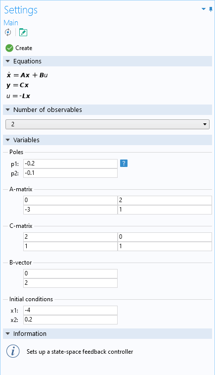
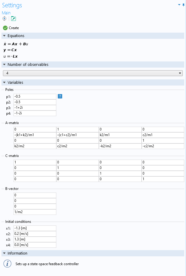
The Settings window for the State-Space Controller add-in.
You define the number of observables to the desired system, as well as the matrices \boldsymbol{A} and \boldsymbol{C}, the vector \boldsymbol{B}, initial conditions, and where to place the poles in a complex plane. The add-in then creates a new 0D model component, which defines the feedback controller using global equations. The Information section mentions the relevant component as well as how to access the output variables once the controller has been created. The control variable is available as u.
Below follows an example of how to use the add-in.
Force Against a Double Mechanical Mass-Damper-Spring Example
Take, as an example, a system describing a point mass of mass m_{1}, attached on the one side to a wall with a spring and a damper, and on the other side to a second point mass of mass m_{2}, also with a spring and damper. The second mass is in turn acted upon by a force, F, which is to be controlled in order to reach equilibrium.
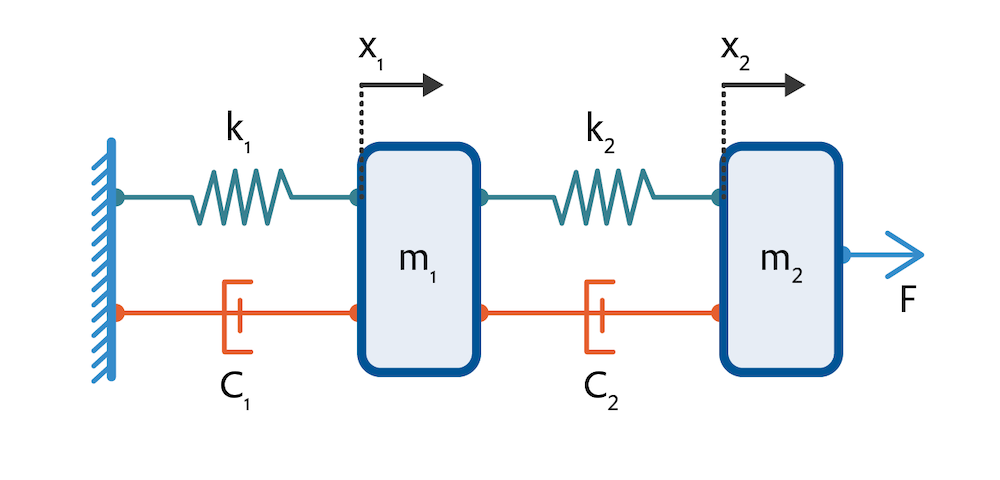
The system is described by the following equations, which are instances of Newton’s second law of motion and where a dot notation is used to indicate time derivatives:
where k_{1} and k_{2} are the spring constants of the two springs, c_{1} and c_{2} are the damping constants of the two dampers, and \tilde{x}_{1} and \tilde{x}_{2} describe the deviation of the two masses from their respective equilibrium position.
Introducing four new variables, x_{1}=\tilde{x}_{1}, \, x_{2}=\dot{\tilde{x}}_{1}, \, x_{3}=\tilde{x}_{2}, and x_{4}=\dot{\tilde{x}}_{2}, we attain a system on the form
with
0 & 1 & 0 & 0\\
-(k_{1}+k_{2})/m_{1}& -(c_{1}+c_{2})/m_{1} & k_{2}/m_{1} & c_{2}/m_{1}\\
0 & 0 & 0 & 1\\
k_{2}/m_{2} & c_{2}/m_{2} & -k_{2}/m_{2} & -c_{2}/m_{2}
\end{pmatrix}, \, \text{ and } \boldsymbol{B} = \begin{pmatrix}
0 \\
0\\
0\\
1/m_{2}
\end{pmatrix}.
In this case, the control variable, u, is the force, F, and \boldsymbol{C} is the identity matrix. We will define constants as parameters, as follows.
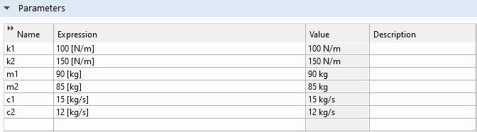
Definition of constants.
We can now use the State-Space Controller add-in to place the poles of the closed-loop system. Assume that we want four real poles, all at -0.5. Since we have four observables, we set up the add-in as shown below.
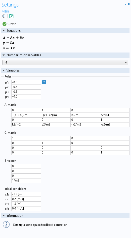
State-space controller setup for the double mechanical mass-damper system.
The initial conditions have been chosen so that the first mass starts 1.3 m in the negative x direction from its equilibrium, with a velocity of 0.2 m/s, and the second mass starts at rest, 1.3 m in the positive x direction from its equilibrium.
By clicking Create, we receive the following message.
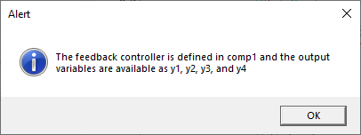
Description of output variables from the state-space controller.
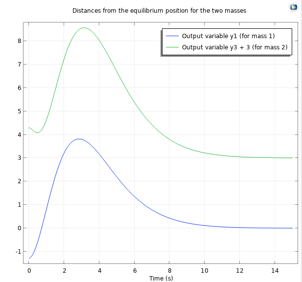
Now, we can run a study and, assuming that the masses are separated by 3 m at equilibrium, we can plot the variables y1 and y3+3 in order to see the time evolution of their position. Since y1 and y3 are the distances from the equilibrium position of the two masses, y3+3 is the distance of Mass 2 from the equilibrium of Mass 1 when the two masses are separated by 3 m.
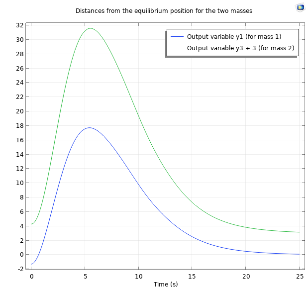
The position of the two masses for the first 25 seconds, when all poles are placed at -0.5.
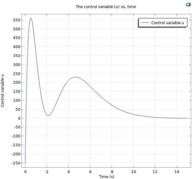
We can also plot the force, which is accessible as the control variable, u. We attain the following plot.
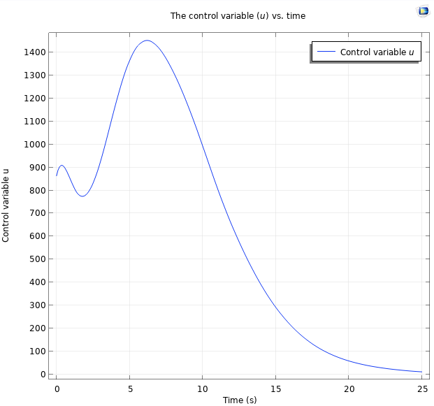
The control variable plotted for the first 25 seconds of the simulation, when all poles are placed at -0.5.
Let’s say that we are not satisfied with the settling time of the above systems. From control theory, we expect the settling time to be reduced if we place the poles further into the negative real plane. If we follow the procedure above, placing all poles at -1 instead of -0.5, we attain the following plot for the positions.
Position plot for the first 15 seconds, when all poles are placed at -1.
Furthermore, we attain the following plot for the controlled force.
Force plot for the first 15 seconds, when all poles are placed at -1.
As expected, the system settles faster.
In the State-Space Controller add-in, there is also the possibility to place poles in the complex plane. Complex poles always come as pairs of complex conjugates.
State-space controller setup with two complex poles.
This results in the following position and control signal plots.


Position plot for two real poles at -0.5, and two complex poles at -1+2i and -1-2i, respectively (left). Control signal plot for two real poles, at -0.5, and two complex poles at -1+2i and -1-2i, respectively (right).
Pole Placement
As seen in the simulations in the previous section, the behavior of the system can change drastically, depending on where the poles of the closed-loop system are placed. It is difficult to find a general description of how the placement of poles affects an arbitrary system. However, it can be said that placing the poles of a continuous system, as the one above, should lead to faster stabilization, but may lead to a larger control signal. Using the State-Space Controller add-in, you can easily evaluate the system behavior for various pole placements.


Comments (4)
Ivar KJELBERG
March 24, 2021Nice Blog Magnus :),
But, what if you could show us the steps how to extract the “reduced state space matrices” directly from a full COMSOL FEM model?
As if we take a simple supported “beam”, actuated by some Force transducer at half length, with the beam tip position measured by some “sensor” probe and we want to control that “mechanism” with a state space controller, we should now be able to extract the reduced state matrices directly from the FEM model, with the model reduction tool, no ?
Then we do not need to rewrite fully all the equations above and enter them manually.
Our previous NASTRAN FEM expert did this some 30 years ago, with brio, but he retired a decade ago … 🙂
We should be able to do it today, with COMSOL too, but I have not found any “procedure” to ensure I do it right, perhaps you may help here Magnus ?
As this is really a very powerful way to get directly from our model the best start of a state space closed loop controller.
Sincerely,
Ivar
Magnus Ringh
March 25, 2021 COMSOL EmployeeHi Ivar, and thanks!
Yes, what you suggest seems like a natural extension of this example. We’ll look into it.
Best regards,
Magnus
Mohammed Alnuaimi
July 12, 2021Hi Magnus,
Thanks for the blog…
Have you and your team found a way to do what Ivar suggested … It will be very helpful if you can provide us with the solution to this problem …
Thank you,
Best Regards,
Mohammed,
Magnus Ringh
July 19, 2021 COMSOL EmployeeHi Mohammed,
The current version of COMSOL Multiphysics is still version 5.6, so the functionality has not changed, but we will be taking your feedback into account when planning additional functionality in future versions of COMSOL Multiphysics.
Best regards,
Magnus