

In this blog post, we investigate syngas combustion in a round-jet burner using the Reacting Flow interface and the Heat Transfer in Solids interface. The results from this benchmark model are compared to experimental findings.
What Is Syngas?
The name syngas gives reference to the role of this fuel gas mixture — comprised mostly of hydrogen, carbon monoxide, and carbon dioxide — as an intermediate in the production process of synthetic natural gas. Syngas, however, is also used to create other products such as methanol, ammonia, and even hydrogen. The idea behind this is a process known as gasification.
In gasification, a solid feedstock is converted to a gas, which can then be used in numerous applications. The gas can be liquefied, for example, by compression. Gasification is particularly valued for its flexibility in the types of feedstock that can be used, with options ranging from coal to biomass. Additionally, this approach simplifies the task of capturing byproducts of the reaction like sulfur or carbon dioxide.
Here, we model syngas combustion in a round-jet burner, comparing our results with experimental data.
Turbulent Combustion of Syngas in a Round-Jet Burner
In the Syngas Combustion in a Round-Jet Burner model, the burner is comprised of a straight pipe within a slow co-flow consisting of air. A gas made up of carbon monoxide, hydrogen, and nitrogen is fed through the pipe with an inlet velocity of 76 m/s (Ma ≈ 0.25). Meanwhile, the co-flow velocity of the air outside of the pipe is 0.7 m/s.
Upon exiting the pipe, the fuel gas mixes with the co-flow, which generates an unconfined circular jet. The turbulent flow of the jet ensures efficient mixing of the two gases and sustains combustion at the exit of the pipe. This is a non-premixed form of combustion as the fuel and oxidizer come into the reaction zone independently.
A schematic of the round-jet burner.
Within this example, we solve for the mass fraction of six chemical species — the five used in the reactions and the nitrogen initially in the co-flow — to model the mass transport in the reacting jet. In the example, the jet features a Reynolds number of around 16700, meaning that the jet is fully turbulent. Because of this, we can assume that the turbulence of the flow has a significant impact on the jet’s mixing and reaction processes.
The k–\omega turbulence model is used to account for this turbulence within the flow field. To model the turbulent reactions, we use the eddy dissipation model, which provides a robust yet simple way of simulating such reactions. Because of heat release in the reactions, there is a significant increase in temperature of the jet — a defining characteristic of combustion. To accurately predict the temperature and composition, we account for the temperature dependence of the species properties as well as the physical properties of the fluid.
The syngas combustion model involves a high degree of coupling, combining turbulent flow with heat and mass transfer. A thorough overview of the solution steps to solve such a non-linear model is shown in the Model Gallery entry.
Simulation Results
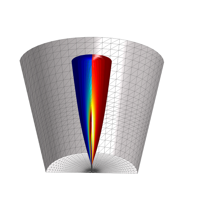
The first figure below depicts the velocity field within the reacting jet, illustrating the expansion and creation of the hot free jet. Within the outer parts of the jet, turbulent mixing prompts the acceleration of fluid initially from the co-flow and brings it into the jet, a process referred to as entrainment. This transition of fluid is evident in the co-flow streamlines that bend towards the jet downstream of the opening of the pipe.
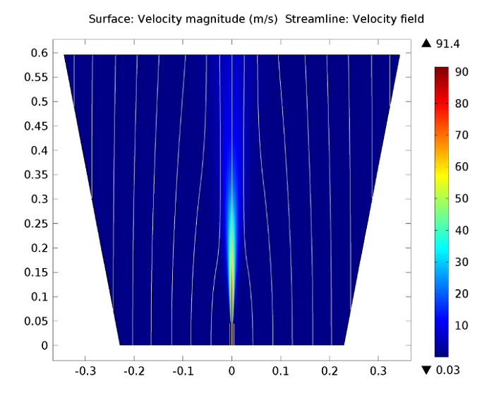
The velocity flow magnitude and field.
Next, we can analyze the temperature in the jet, using a revolved data set to visualize the model in full 3D. Here, we identify the maximum temperature within the combustion region as about 1960 K.
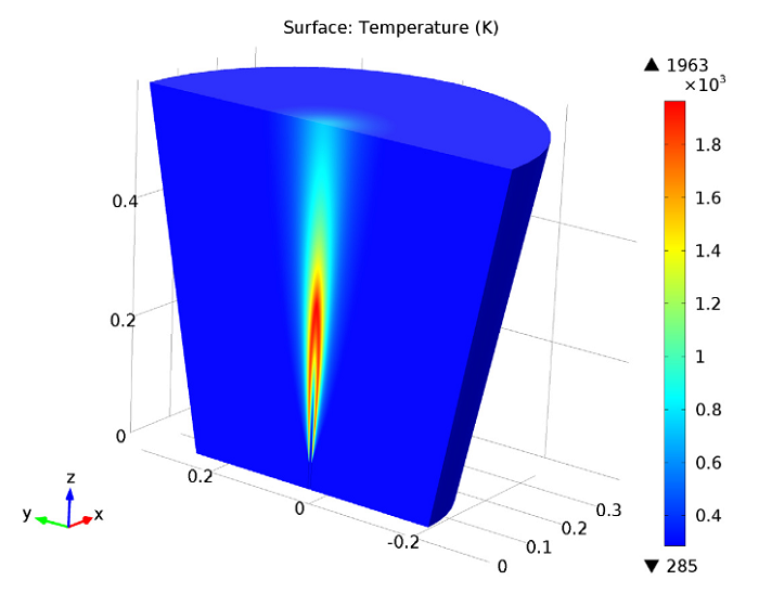
Jet temperature.
The following figure illustrates the carbon dioxide mass fraction within the reacting jet. CO2 is formed in the jet’s outer shear layer, right outside of the pipe. It is in the outer shear layer that the fuel reacts with the oxygen in the co-flow, with turbulent mixing encouraging the reactions. Like the CO2 formation, the temperature increase depicted in the previous plot also takes place just outside of the pipe. This suggests no lift-off and the attachment of the flame to the pipe.
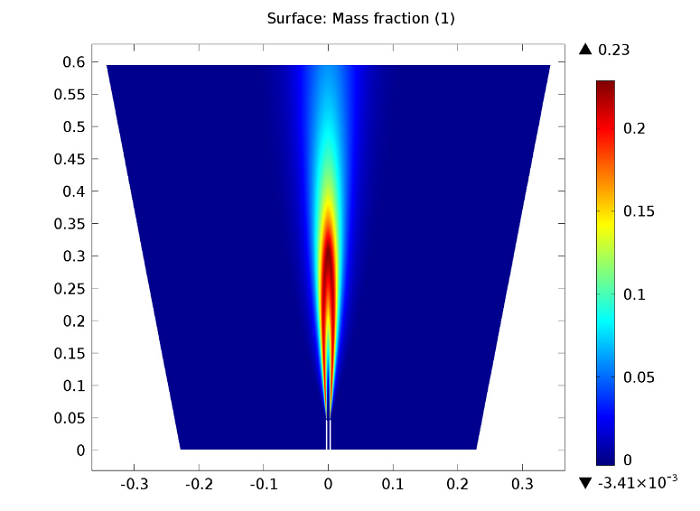
Carbon dioxide mass fraction.
Simulation Results vs. Experimental Data
Let’s now shift our focus to comparing the simulation results with experimental data. Our analysis begins with the jet temperature profiles along the centerline, as shown in the figure on the left, below. In this graph — and the ones that follow — lines represent the model results and symbols are used to indicate the experimental values. The plot of the centerline shows that the maximum temperature predicted in the model is close to that from the experimental results.
In the model results, you may notice that the temperature profile shifts in the downstream direction. This difference can be attributed to the fact that radiation has been left out of the model. Meanwhile, the figure on the right compares the temperature profiles along a horizontal line at two different positions (20 and 50 pipe diameters) downstream of the pipe exit. Again, there is a good agreement between the values obtained in the simulation and those from the experiment.
")
Left: A plot comparing jet temperatures along the centerline. Right: Jet temperatures at 20 and 50 pipe diameters downstream of the pipe exit.
When comparing the axial velocity of the jet with experimental data, we can observe that these results are in excellent agreement for both positions (20 and 50 pipe diameters). This is illustrated here:
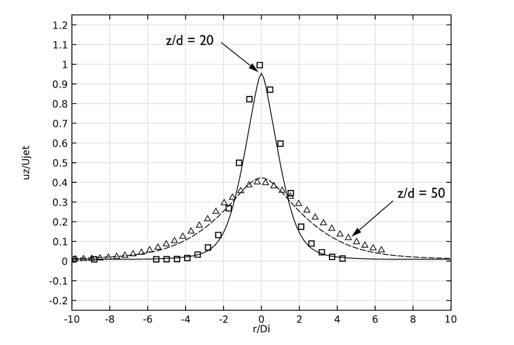
Axial velocity at the same downstream positions as the previous plot.
Lastly, we evaluate the species concentration along the jet centerline. In the case of the species N2 and CO, the axial mass fraction development aligns closely with experimental data. H2O and H2 are found to agree fairly well with the experimental values, with a slight shift on H2O. The species CO2 and O2 feature a similar trend as the experimental results but, just as in the temperature, the profiles are found to shift downstream. Here, the discrepancy can be somewhat attributed to the lack of inclusion of radiation in the model. However, the simplified reaction scheme and the eddy dissipation model are likely to have an influence on the accuracy as well.
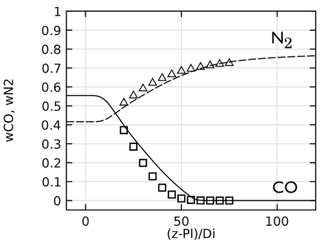
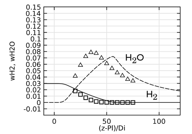
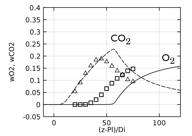
Comparing species mass fractions along the jet centerline.
Try It Yourself
- Download the model: Syngas Combustion in a Round-Jet Burner


Comments (0)