

In a previous blog post, we discussed the physiological basis of generating action potential in the excitable cells of living organisms. We spoke about the simple Fitzhugh-Nagumo model, which emulates the process of depolarization and repolarization in a cell’s membrane potential. Today, we analyze a more advanced model for simulating action potential, the Hodgkin-Huxley model. We also go over how to use a computational app to streamline this type of analysis.
Exploring Action Potential in Cells with the Hodgkin-Huxley Model
We have already gone over the physical basis of the firing mechanism that generates action potential in cells and we studied the generation of such a waveform using the Fitzhugh-Nagumo (FH) model.

The dynamics of the simple Fitzhugh-Nagumo model, featured in a computational app.
Today, we will convert the FH model study into a more rigorous mathematical model, the Hodgkin-Huxley (HH) model. Unlike the Fitzhugh-Nagumo model, which works well as a proof of concept, the Hodgkin-Huxley model is based on cell physiology and the simulation results match well with experiments.
In the HH model, the cell membrane contains gated and nongated channels that allow the passage of ions through them. The nongated channels are always open and the gated channels open under particular conditions. When the cell is at rest, the neurons allow the passage of sodium and potassium ions through the nongated channels. First, let us presume that only the potassium channels exist. For potassium, which is in excess inside the cell, the difference of concentration between the inside and outside of the cell acts as a driving force for the ions to migrate. This is the process of movement of ions by diffusion, or the chemical mechanism that initially drives potassium out of the cells.
This movement process cannot go on indefinitely. This is because the potassium ions are charged. Once they accumulate outside the cell, these ions establish an electrical gradient that drives some potassium ions into the cells. This is the second mechanism (the electrical mechanism) that affects the movement of ions. Eventually, these two mechanisms balance each other and the potassium efflux and outflux balances. The potential at which the balance happens is known as the Nernst potential for that ion. In excitable cells, the Nernst potential value for potassium, E_{K}, is -77 mV and for sodium ions, E_{Na}, is around 50 mV.
We allow the presence of a few nongated sodium channels in the membrane. Because the sodium ions abound in the extracellular region, an influx of sodium ions into the cell must occur. The incoming sodium ions reduce the electrical gradient, disturb the potassium equilibrium, and result in a net potassium efflux from the cell until the cell reaches its resting potential at around -70 mV. It is important to mention here that the net efflux of potassium and net influx of sodium ions cannot go on forever, otherwise the chemical gradient that causes the movement will eventually cease. Ion pumps bring potassium back into the cell and drive sodium out through active transport and maintain the resting potential of the cells in normal conditions.
Let’s derive an equivalent circuit model of a cell in which we can imitate the effects of the different cellular mechanisms we just described by different commonly found circuit components, such as capacitors, resistors, and batteries. The voltage response of the circuit is the signal that corresponds to the action potential.
Overall, there are four currents that are important for the HH model:
- The current that flows into the cell membrane
- A sodium current
- A potassium current
- A leak current that accounts for any other current, except for the first three
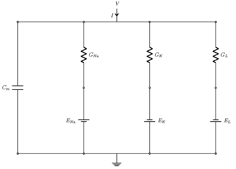
Schematic of the currents in a Hodgkin-Huxley model.
The four currents flow through parallel branches, with the membrane potential V as the driving force (see the figure above; the ground denotes extracellular potential). The cell membrane has a capacitive character, which allows it to store charge. In the figure above, this is the left-most branch, modeled with a capacitor of strength Cm. The other branches account for three ionic currents that flow through ion channels. In each branch, the effects of channels are modeled through conductance (shown as resistance in the diagram), and the effect of the concentration gradient is represented by the Nernst potential of the ions, which are represented as batteries.
Thus, when a current is injected in the cell, it gets divided into four parts and the conservation of charges leads us to the following balance equation
Or equivalently
What is of paramount importance is that the sodium and potassium channel conductances are not constant; rather, they are functions of the cell potential. So how do we model them? Remember that some of the ion channels are gated and they can have multiple gates. Assume that there are voltage-dependent rate functions αρ (V) and βρ (V), which give us the rate constants of a gate going from a closed state to open and open to closed, respectively. If ρ denotes the fraction of gates that are open, a simple balance law yields the following equation for the evolution of ρ
Different gated channels are characterized by their gates. In the HH model, the potassium channel is hypothesized to be composed of four n-type gates. Since the channel conducts when all four are open, the potassium conductance is modeled through the equation
For sodium, the situation is assumed to be more complicated. The sodium-gated channel has four gates, but three m-type gates (activation-type gates that are open when the cell depolarizes) and one h-type gate (a deactivation gate that closes when the cell depolarizes). Therefore, the sodium channel conductance is given by
In the above equations, \bar{g}_{K}, \bar{g}_{Na} is the maximum potassium and sodium conductance. The functional forms of αρ (V), βΡ (V) for p =m, n, h can be found in any standard reference.
The leak conductance is assumed to be a constant. Therefore, the HH model is completely described by the following set of equations
C_m\frac{dV}{dt} &= I-\bar{g}_{Na}m^3h(V-E_{Na})-\bar{g}_{K}n^4(V-E_{K})-g_{L}(V-E_L), \\
\frac{dm}{dt} &= \alpha_m \left(V\right) \left(1-m \right) + \beta_m\left(V\right) m,\\
\frac{dn}{dt} &= \alpha_n \left(V\right) \left(1-n \right) + \beta_n\left(V\right) n,\\
\frac{dh}{dt} &= \alpha_h \left(V\right) \left(1-h \right) + \beta_h\left(V\right) h.
\end{aligned}
Understanding the Dynamics of the HH Model with Simulation
The key to understanding the Hodgkin-Huxley model lies in understanding the gate equations. We can recast the equations for the gates in the following form
with p_{\infty}\left(V\right) = \frac{\alpha_p\left(V\right)}{\alpha_p\left(V\right) + \beta_p\left(V\right)}, \quad \tau_p\left(V\right) = \frac{1}{\alpha_p\left(V\right) + \beta_p\left(V\right)}.
This is a very well-known equation in electrical circuits. If we assume ρ∞ is voltage independent, then the equation says that ρ asymptotically approaches ρ∞ as its final value, and Τρ, the time constant, dictates the rate of approach. This means that the smaller the Τρ, the faster the approach. The following figure shows the values of these two quantities for p =m, n, h.


The asymptotic values (left) and time constants (right) for the gate equations of the Hodgkin-Huxley model.
It is easy to conclude from the figures above that n∞, m∞ increases as the cell depolarizes and h∞ decreases under similar conditions. From the second graph, we find that the activation for sodium is much faster compared to the activation of potassium or the leak current.
When depolarization starts, n∞, m∞ increases and h∞ decreases. The governing equations of all of these quantities demand that they should approach the steady-state values; therefore, n, m increases and h decreases. However, we should also remember the differences in time constants of the gating variables. A comparison says that the activation of sodium gates happens much faster as compared to their deactivation or the opening of potassium channels. Therefore, there is an initial overall increase in the sodium conductance. This results in an increase of the sodium current, which raises the membrane potential and causes V to approach E_{Na}. This is how the HH model accounts for the rising part of the action potential.
However, as this process continues, h \rightarrow 0. Once the value of h goes below a threshold, the sodium channels are effectively closed. Also, the approach of V toward E_{Na} kills the driving force for the sodium current. Meanwhile, the potassium channels, which have a slower time constant, open up to a large extent. This, coupled with the large driving force V-E_{k} that is available for the potassium current, forces the reverse flow. The potassium ions move out of the cell and eventually the membrane potential settles toward the hyperpolarized state.
Building and Using a Simulation App to Analyze the Hodgkin-Huxley Model
We can build a computational simulation app to analyze the Hodgkin-Huxley model, which enables us to test various parameters without changing the underlying complex model. We can do this by designing a user-friendly app interface using the Application Builder in the COMSOL Multiphysics® software. As a first step, we create a model of the Hodgkin-Huxley equations using the Model Builder in the COMSOL software. After building the underlying model, we transform it into an app using the Application Builder. By building an app, we can restrict and control the various inputs and outputs of our model. We then pass the app to the end user, who doesn’t need to worry about the model setup process and can focus on extracting and analyzing the results of the simulation.
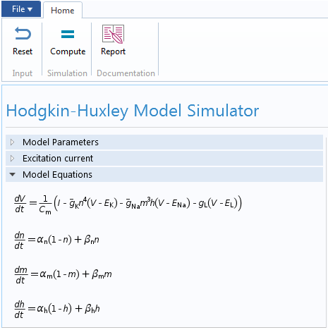
In our case, we implemented the underlying Hodgkin-Huxley model using the Global ODEs and DAEs interface in COMSOL Multiphysics. This interface is a part of the Mathematics features in the COMSOL software and is capable of solving a system of (ordinary) differential-algebraic equations (Global ODEs and DAEs interface). This interface is often used to construct models for which the equations and their initial boundary conditions are generic. In the interface, we can specify the equations and unknowns and add initial conditions. The interface, with model equations, is shown below.

We also create the postprocessing elements, graphs, and animations in the Model Builder. Once the model is ready, we move on to the Application Builder again. We connect the elements of the model to the app’s user interface through various GUI options like input fields, control buttons, display panels, and some coded methods.
You can learn more about how to build and run simulation apps in this archived webinar.
Finally, we can design the user interface of the Hodgkin-Huxley app. With the Form Editor in the Application Builder, we can design a custom user interface with a number of different buttons, panels, and displays. This user interface features a Model Parameters section to input the different parameters of the HH model, such as the Nernst potential, maximum gate conductance, and membrane capacitance. We can also provide two types of excitation current to the model: a unit step current or an excitation train. As the parameters change, the app displays the action potential and excitation current, as well as the evolution of gate variables m, n, and h.
With the Reset and Compute buttons, it is easy to run multiple tests after changing the parameters. There are also graphical panels that display visualizations and plots of the model results. The Report button generates a summary of the simulation.

The user interface for the Hodgkin-Huxley Model simulation app.
Making buttons work in an app is a simple process. All we have to do is write a few methods using the Method Editor tool that comes with the Application Builder and connect them to the buttons properly. Let me illustrate with an example. We can design the Hodgkin-Huxley Model app so that when it launches, the Report button is inactive (see the figure below). This is because the app user will not need to use this button until after they perform a simulation.
The Report button is disabled at the start of the simulation.
To do so, we can write a method that instructs the app to execute certain functions during the launch.
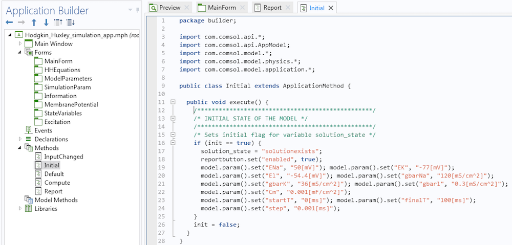
A method that disables the Report button during launch.
Observe that we have disabled the Report button using instructions in lines 7 and 8 in the method. If you are worried about coming up with the syntax for your methods, let me assure you that it is much more simple than it seems. First, the methods execute some actions. If we want to record the code corresponding to these actions, we click on the button called Record Code in the Application Builder ribbon. Then, we can go to the Model Builder, execute the actions, and once done, click on the Stop Recording button. The corresponding code will be placed in the method. If necessary, we can then modify the instructions.
Once a simulation is complete, we would like this button to become active in the app. In another method associated with the Compute button, we insert the following code segment
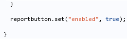
We then ensure that this segment is executed if the solution is computed successfully. You will see that this enables the button.
To summarize, you can use a simulation app to easily compute and visualize parameter changes when working with a complex model that involves multiple equations and types of physics, such as the Hodgkin-Huxley model discussed here. This simulation app is just one example of how you can design the layout of an app and customize its input parameters to fit your needs. Use this app as inspiration to build your own app, whether you are analyzing the action potential in a cell with a mathematical model or teaching students about complicated math and engineering concepts. No matter what purpose your app serves, it will ensure that your simulation process is simple and intuitive.
Further Resources
- On the COMSOL Blog:
- Read a previous blog post on exploring the dynamics of the Fitzhugh-Nagumo model with a simulation app
- Learn more about using simulation apps to streamline your modeling process
- Browse upcoming live webinars to learn more about the features and functionality within COMSOL Multiphysics


Comments (1)
Kris Carlson
February 24, 2017Hi – per note to Amlan please send me the mph file (not the app) so that I can compare his implementation of the Hodgkin-Huxley model to ours and others’. Thank you.
Kris (kris@kriscarlson.com)