

The reduction of aircraft engine noise has been a priority in the aviation industry for many years. Minimizing sound emissions, of course, requires an understanding of engine noise — a task that can become quite challenging due to the complex nature of aircraft systems and geometries. Using a model of an aero-engine duct, we provide a more in-depth look at the acoustical field in aircraft engines.
What’s All That Noise About?
Whether on your way to the airport or simply passing by one, you have likely experienced watching a plane fly right overhead as it prepares to land. It is often a sight at which we marvel, to see a plane flying so low to the ground, but another element that can be quite captivating is the sound that the aircraft makes. While our experience lasts only for a short moment, imagine what it is like for those residents living in close proximity to the airport, hearing that sound periodically throughout the day. Taking this perspective, it is easy to see why addressing aircraft noise has become such a prevalent area of concern.
Since becoming a public issue in the 1960s, new regulations and research have initiated the development of quieter aircraft. One design element that has proven successful within this movement is a high-bypass turbofan engine. Used in the majority of airliners, these engines feature a fan that captures incoming air. As the air passes through the fan, a portion enters the combustion chamber, while the remainder bypasses the engine. Compared to its predecessor, the turbojet, in which all air passes through the gas generator, the turbofan engine creates less aircraft engine noise while also offering greater thrust at lower speeds.
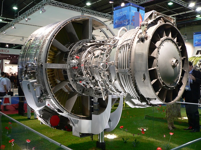
A CFM56 turbofan engine. (“CFM56 P1220759” by David Monniaux — Own work. Licensed under Creative Commons Attribution Share-Alike 3.0, via Wikimedia Commons).
With this improved engine technology, the next step becomes analyzing the acoustical field of the turbofan engine in an effort to optimize its design. For this, we can turn to simulation.
Modeling of Aircraft Engine Noise
To analyze aircraft engine noise, we can use the Flow Duct model in COMSOL Multiphysics. This model features an axially symmetric duct within a turbofan engine. It is an approximate model of a turbofan’s inlet section in the CFM56 series (which is quite common among airliners). In this example, it is assumed that the flow of air is compressible, irrotational, has no viscosity, and constant entropy. The acoustic field is modeled as perturbations on top of the background flow using the linearized potential flow equations. With these formulations, the pressure and the velocity field are directly related to and derived from a so-called velocity potential.
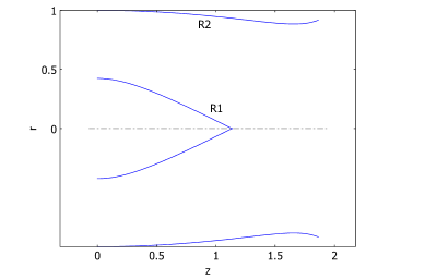
The geometry of the duct.
In this model, z = 0 is referred to as the source plane and represents the fan’s location in the actual geometry of the engine. A noise source is introduced at this boundary. Meanwhile, z = L represents the engine’s fore end and is known as the inlet plane. Variables R1 and R2 indicate the spinner and duct-wall profiles.
In this study, we model cases with and without a compressible irrotational background flow. With Mach number M = -0.5 (flow in the negative z-direction) and M = 0 (no flow), respectively. The analysis also compares the use of hard and lined walls within the duct.
The Results
The model first solves the background flow, which is assumed to be stationary. Then, a suitable acoustic source (a given propagating eigenmode) is derived. Finally, the acoustic field is found.
For the case with a mean background flow (M = -0.5), the velocity potential was found to be uniform beyond the terminal plane (contour lines in the plot below). Additionally, the deviations in the mean density value (due to the compressible nature of the air flow) were most prevalent in nonuniform areas of the duct’s geometry, such as the tip of the spinner. These deviations are highlighted by the red and blue colors in the figure below.
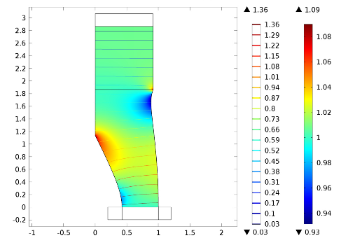
Plot of mean-flow field for source plane M = -0.5. The color surfaces correspond to the background density and the contour plots to the velocity potential.
Using these results, we can then calculate eigenmodes for the acoustic field at the source of the noise. These can be shown to represent a certain component of the engine noise source at a given frequency. The graph below shows the resulting velocity-potential profile for the first axial boundary mode at the source plane in the case of M = -0.5 and M = 0.
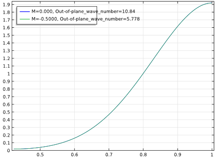
Graph showing the resulting velocity-potential profile for the lowest mode.
With the background flow and a source at hand, the acoustic field can now be solved for. The results (seen below) can be compared to results for a similar system presented by Rienstra and Eversman (2001).
In the cases without a background flow, the acoustic pressure distribution for both hard and lined walls were in good agreement when compared to the simulation results in the paper. With the mean flow, the results from the hard wall case paired well with alternate solutions. However, in the case of the lined wall, there were some notable differences, specifically near the source plane. These differences can be explained by the discrepancy in the noise source definition. In this model, the source mode was derived for the hard duct wall case, while the compared simulation used a noise source adapted to the acoustic lining.
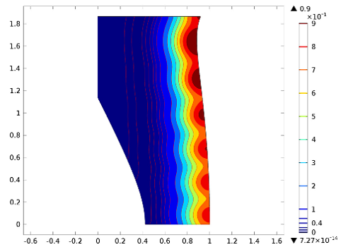
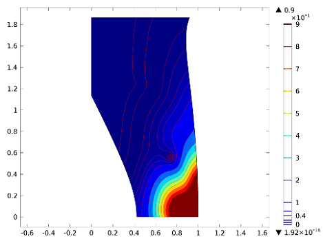
Pressure distribution in the acoustic field for hard (top) and lined (bottom) duct wall in cases with no mean flow (M = 0).
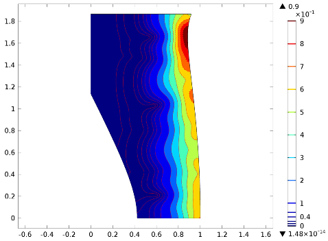
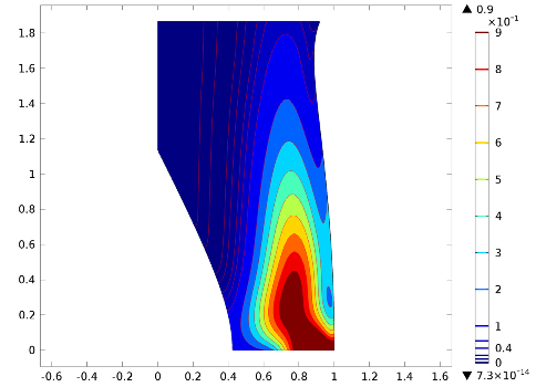
Pressure distribution in the acoustic field for hard (top) and lined (bottom) duct wall in cases with a mean flow (M = -0.5).
The model presented here is very conceptual, but it could potentially be extended for more complex situations. By modeling these systems, it is possible to optimize the shape of certain engine duct parts and the lining properties in order to reduce the sound emission. Such optimization should, of course, go hand-in-hand with a control of the flow properties in order to not degrade the engine’s performance.
Further Reading
- Try it yourself: Download the Flow Duct model now.
- S.W. Rienstra and W. Eversman, “A Numerical Comparison Between the Multiple-Scales and Finite-Element Solution for Sound Propagation in Lined Flow Ducts,” J. Fluid Mech., vol. 437, pp. 367–384, 2001.

Comments (0)