

Today, guest blogger and Certified Consultant Ionut Prodan of Boffin Solutions, LLC discusses using a hybrid approach to calculate fracture flux in thin structures.
When modeling thin fractures within a 3D porous matrix, you can efficiently describe their pressure field by modeling them as 2D objects via the Fracture Flow interface. Significant fracture flux calculation issues, however, may arise for systems of practical interest, such as hydraulic fractures contained within unconventional reservoirs. See how a hybrid approach overcomes such difficulties.
From 3D to 2D: Modeling Thin Fractures
To model an actual fracture as a 2D object using the Subsurface Flow Module, you first have to solve for the pressure field (through a tangential form of Darcy’s law) within the internal surface representing the fracture’s lateral extent. You can then calculate, in principle, the corresponding fluid flux through the actual fracture cross section by multiplying the component normal to an edge of the velocity vector (delimiting the 2D fracture object) by the fracture’s thickness. This approach is much more computationally efficient, as a very thin but otherwise ample 3D object can now be described as a 2D object, one that only needs to be meshed as a surface.
Say you have a 2D fracture object with the following characteristics:
- It has an edge contained within the porous matrix.
- It is significantly more permeable than its surrounding formation.
- It features a very large aspect ratio between its lateral and cross-sectional dimensions.
In a system of interest such as this, significant fracture flux computational errors can occur. Let’s take a look at one such example.
Note: With the latest version of the COMSOL Multiphysics® software — version 5.2a — you can also model heat transfer in thin fractures. This is made possible via the Heat Transfer in Fractures interface.
Addressing Fracture Flux Computational Errors: A Reservoir Block Example
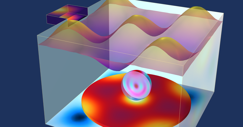
The system shown below features a 3D penny-shaped hydraulic fracture embedded in a reservoir block and connected to a horizontal well. The inlet for this simplified system consists of the two reservoir boundaries shown in green at the top and the back of the block. The only outlet is through the narrow boundary where the fracture disc connects to the wellbore. Both the inlets and the outlet are set as pressure boundary conditions, with the values of ΔP and 0, respectively. The geometry only considers one quarter of the actual system, as it takes advantage of existing symmetry.
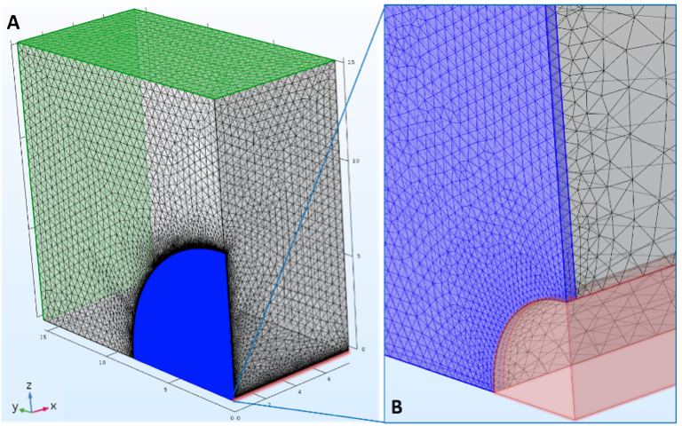
A 3D penny-shaped fracture (shown in blue) embedded in a reservoir block and hydraulically connected to a horizontal well (shown in red). The two reservoir inlet boundaries are highlighted in green.
Note that the dimensions of the above system are not representative of cases of practical interest. The dimensions are scaled down to allow for adequate 3D meshing of the discoidal fracture, which has a radius of 7.62 m (25 ft) and a thickness d_{HF} of 1.27 cm. (Properly meshing 3D fractures with radii of hundreds of feet, as encountered in field applications, would be quite computationally expensive.) The wellbore radius is 12.7 cm (5 in), while the reservoir block’s dimensions are approximately 8 m x 15 m x 15 m (25 ft x 50 ft x 50 ft). The entire mesh consists of 2,246,298 tetrahedral elements, 657,720 of which are used for the discoidal fracture domain alone. The minimum and average element quality values of the latter are 0.148 and 0.700, respectively, while the average quality for the entire mesh is 0.673.
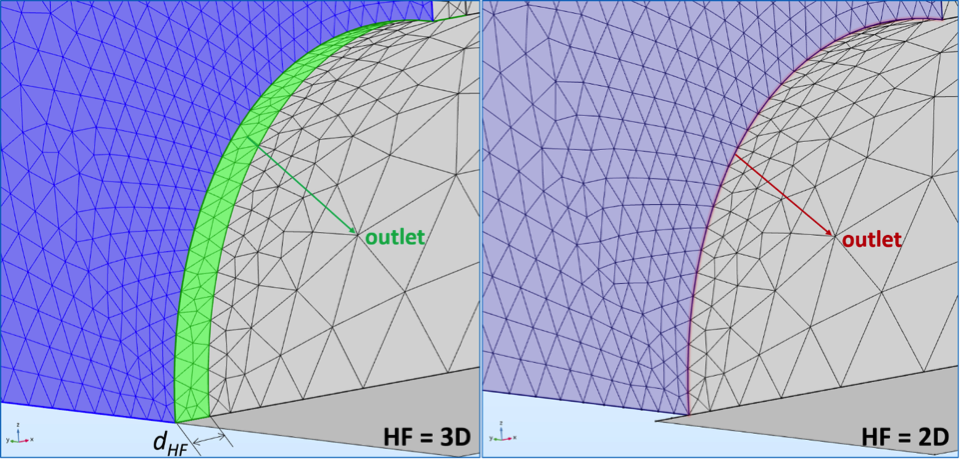
Outlet boundaries for the 3D (shown in green) and 2D (shown in red) realizations of the actual hydraulic fracture of thickness dHF.
Darcy’s law {\overrightarrow{u}}=-\frac{K}{\mu} \nabla p is used to solve for the pressure field p in incompressible, single-phase, and stationary flow parametric studies for various values of the drawdown ΔP. The fluid is a light liquid hydrocarbon with a dynamic viscosity \mu value of 0.26 cP. The permeability of the reservoir matrix is taken as 1 mD, while that of the (propped) hydraulic fracture is 45.6 Darcy.
The fracture flux calculation issue referenced above is depicted in the following figure. This figure shows the inlet and outlet flow rates as functions of the drawdown ΔP when the hydraulic fracture (HF) is described as either a 3D or 2D object. While the first three curves (for the inlet flow rates and the 3D outlet flow rate) overlap as expected, the outlet flow rate for the 2D case represents only a quarter of the inlet flow rate. The fluxes for the first three curves were calculated as integrals of the normal component of the fluid velocity vector {\overrightarrow{u}} over the respective inlet and outlet surfaces (\smallint\smallint {\overrightarrow{u}} \cdot {\hat{n}} ̂dA〗). The outlet flow rate for the 2D fracture, meanwhile, was calculated as an integral of {\overrightarrow{u}} \cdot {\hat{n}} along the outlet edge, multiplied by the fracture thickness dHF: Q_{Out}^{2D}=d_{HF} \smallint {\overrightarrow{u}} \cdot {\hat{n}} ̂dl〗.
The Q_{Out}^{2D} flux calculation issue remains regardless of the applied meshing and no matter how \smallint {\overrightarrow{u}} \cdot {\hat{n}} ̂dl〗 is probed, with its integrand expressed as (dl.nx*dl.u + dl.ny*dl.v + dl.nz*dl.w), (sys1.e_n1*dl.u + sys1.e_n2*dl.v + sys1.e_n3*dl.w), dl.bndflux/dl.rho, or as (root.nx*dl.u + root.ny*dl.v + root.nz*dl.w). The ‘dl.’ identifier stands for the applied interface (Darcy’s Law interface); {nx,ny,nz} are the Cartesian components of the unit vector normal to the edge {\hat{n}}〗; and {u,v,w} are the Cartesian components of the fluid velocity vector {\overrightarrow{u}}.
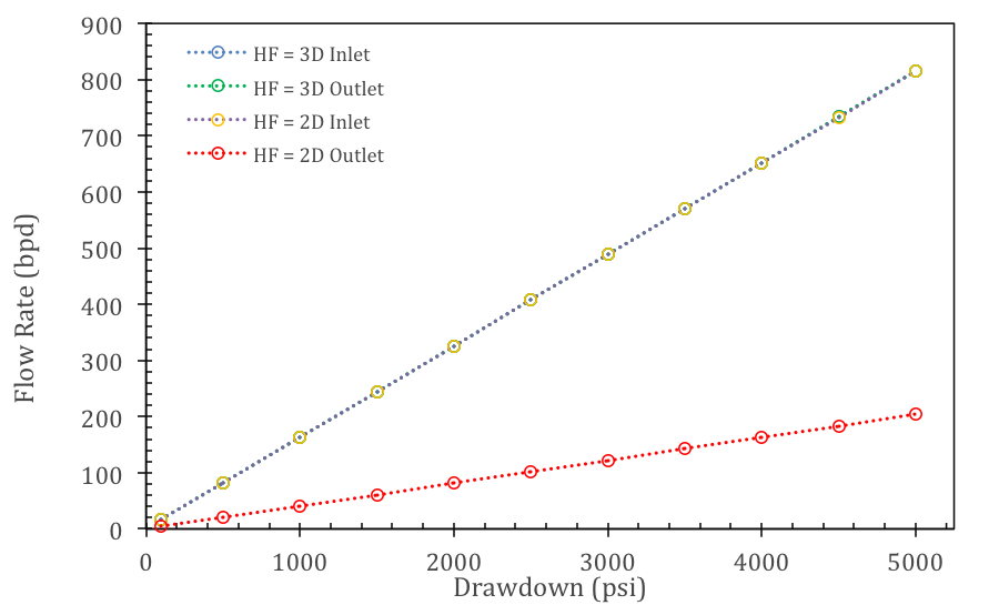
Inlet and outlet flow rates as functions of the drawdown ΔP when the actual HF is modeled as either a 3D or 2D object for the respective system.
Notice that when the hydraulic fracture is described as a 2D object, the discoidal fracture (3D) domain is omitted from the model and is considered instead only through its inner lateral boundary. Otherwise, the geometry and mesh are identical between the 2D and 3D descriptions. This simplification greatly reduces the size of the system and thus represents one of the most attractive elements of the Fracture Flow interface: it enables the modeling of much larger fracture surfaces with proper meshing. As such, it would be quite useful if there was a way to work around the 2D fracture outlet flux issue.
Overcoming Fracture Flux Conservation Issues with a Hybrid Approach
A hybrid approach, which combines a 2D description of the fracture away from the wellbore with a 3D one in its immediate vicinity, makes this possible. The figure below shows the meshed geometry of the hybrid implementation. The 3D component of the fracture is represented by the blue domain, while the 2D component is represented by a red surface, which depicts the boundary toward the porous matrix of the actual fracture. Note that the 3D part of the actual fracture that corresponds to the 2D component is excluded from the model.
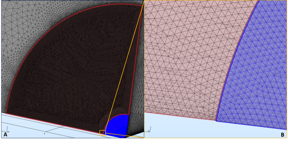
Meshed geometry of the hybrid fracture implementation. The blue domain represents the 3D component of the fracture, while the red surface represents the 2D component. The latter is chosen as the inner lateral boundary of the actual fracture (toward the matrix).
In the hybrid approach, the pressure field continues to be properly accounted for at any point within the actual fracture, while the flux through the outlet boundary is computed without the shortcoming of the 2D description. The following table compares relevant quantities for the 3D, 2D, and hybrid realizations of the hydraulic fracture. These computations were performed using a direct solver on a machine with an Intel® Core™ i74770 processor and 32 GB RAM.
| Hydraulic fracture | Degrees of freedom | Memory (GB) | Time per iteration (s) | Q_{in}/Q_{in}^{3D} | Q_{out}/Q_{in}^{3D} |
|---|---|---|---|---|---|
| 3D | 3,231,747 | 23.74 | 247.5 | 1 | 1.00026 |
| 2D | 2,354,490 | 15.98 | 153.5 | 0.99948 | 0.24992 |
| Hybrid | 2,397,891 | 16.50 | 158.0 | 0.99941 | 0.99967 |
Comparison of relevant quantities for the 3D, 2D, and hybrid realizations.
The plot below shows, in logarithmic scale, the pressure profiles along a diagonal line within the YZ-plane containing the 2D fracture surface for a drawdown of 100 psi. This probe line is delimited by the outlet (wellbore) at the lower-right part of the surface and by the inlet of the reservoir block at the other end. The white line at the inset of the plot highlights the probe line. The surface color of the inset corresponds to the pressure value within the probed YZ-plane, and the guiding arrows help map important graphing points on it. The graph’s curves overlap for all three cases, indicating that the pressure field solution is practically identical among the three fracture descriptions: 3D, 2D, and hybrid.
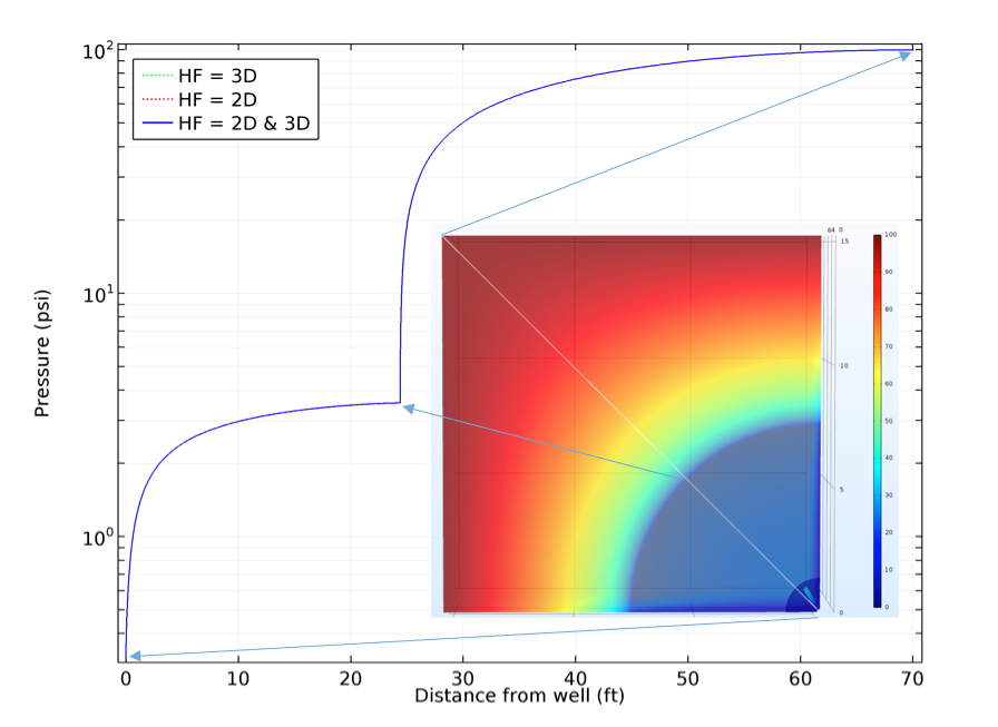
Pressure profiles along a face diagonal line within the YZ-plane.
Hybrid Approach Offers Greater Ease in Modeling Thin Fractures
Flux calculation issues can occur with a solely 2D description of a fracture. As we’ve demonstrated here today, the proposed hybrid approach for describing an actual fracture provides a viable solution. As such, this technique can be applied to various systems of practical interest that feature a greater number of arbitrarily thin fractures.
About the Guest Author

Ionut Prodan is the principal of Boffin Solutions, LLC, a COMSOL Certified Consultant. Prior to his founding of Boffin Solutions, Ionut worked within upstream technology at Shell and Marathon Oil. He earned his doctorate in physics from Rice University, where he conducted research on the photoassociation of ultra-cold atoms and computational solid-state chemistry.
Intel and Intel Core are trademarks of Intel Corporation or its subsidiaries in the U.S. and/or other countries.


Comments (2)
Li Chaeles
June 15, 2017Thanks Ionut!
Nice application. Just want to check is it possible to share the model file?
Ionut Prodan
June 16, 2017Thank you Li.
We could discuss about this by email or phone.
My contact information can be found online at boffin.solutions