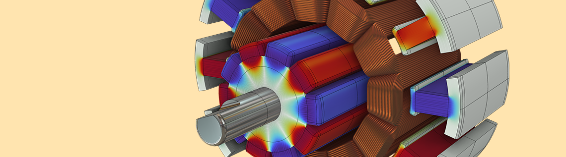

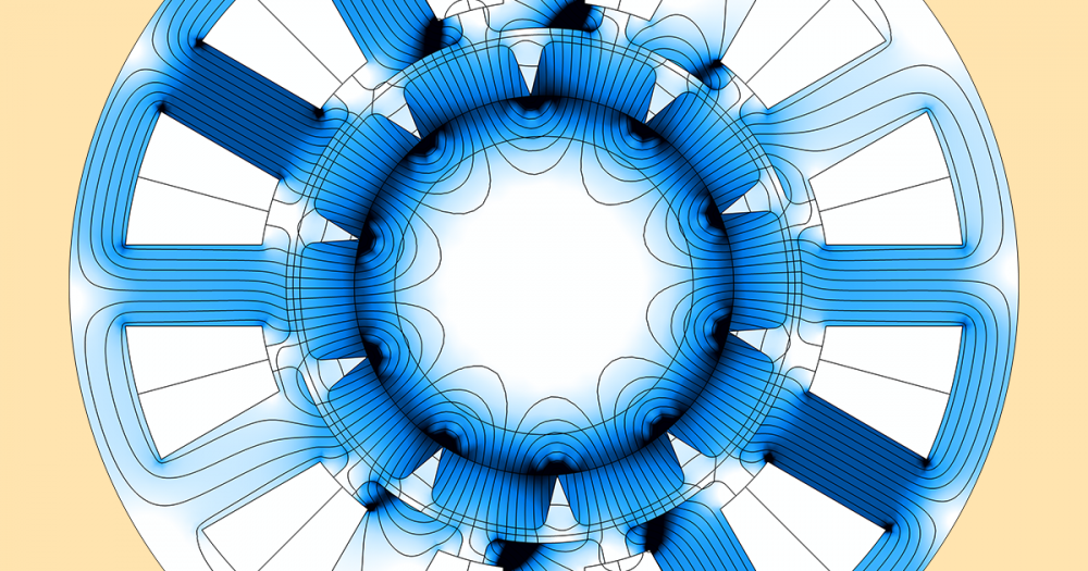
We previously discussed analyzing electric motor and generator designs in the COMSOL Multiphysics® software, including how to examine the magnetic flux distribution, torque, losses, and iron usage in a rotating machine. We used an example of a 12-slot, 10-pole permanent magnet machine (PMM) with a diameter of 35 mm and axial length of 80 mm. In this blog post, we will investigate the variation of iron and copper losses, the resulting temperature rise, and its effect on the efficiency of the PMM. Since we are going to talk about losses, let’s begin by taking a look at a very fundamental aspect of rotating machine simulation: energy conservation.
This is the second blog post in a series discussing how to analyze different design aspects of rotating machines using COMSOL Multiphysics. Read Part 1 here.
Verification of Power Balance
Energy conservation can be examined by checking the relevant power values. For this, we will have a look at the power balance phenomenon in the context of rotating machine simulations. While modeling rotating machines, the stator and rotor iron are typically assigned a zero electrical conductivity, and the iron losses are computed separately using empirical models like Steinmetz or Bertotti. This is because the stator and rotor iron consist of stacks of laminations to minimize eddy currents.
If the bulk conductivity of iron were used, the numerical model would greatly overestimate the losses and compute a low net magnetic field; corresponding to nonlaminated iron. That is why iron losses need to be computed separately. Using this approach, the efficiency can be calculated as \textrm{Efficiency} = \frac{\textrm{Mechanical output power}}{\textrm{Mechanical output power + iron losses + copper losses}}. Here, we have chosen to neglect the friction and windage losses, since we know they constitute only a small fraction of the total loss (about 3%). When deemed necessary, these terms can easily be included.
The information above implies that in electromagnetic FEM simulations, the electrical power input should be used to excite the magnetic fields, produce the torque on the rotor, and generate the copper loss. In terms of energy conservation, the electrical energy input should equal the sum of the mechanical power output and the copper loss. The instantaneous electrical power is given by P_i = V_a I_a + V_b I_b + V_c I_c, where V_a, V_b, V_c and I_a, I_b, I_c are the stator’s three-phase voltages and currents, respectively. The mechanical output power is given by P_o = T_r \omega_r, where T_r is the torque on the rotor and \omega_r is the angular velocity.


Left: The instantaneous power balance for a rotor speed of 3250 rpm and stator current of 10 A. Right: Averaged power balance (the relative error between input power and the sum of output power and copper losses).
The instantaneous power balance can be examined by observing how the mechanical power output, the copper loss, their sum, and the electrical power input vary with time. To investigate the power balance further, the time average of the electrical power input and the sum of output power and copper losses are obtained, for various combinations of rotor speed and stator current. The relative error between the input power and output power plus loss is calculated. The maximum relative error evaluates to less than 1% over the entire range of variation. The power balance verification ensures that no unintended losses are present and gives us confidence in using numerical analysis as a tool for rotating machine development.
Investigating Iron and Copper Losses
Computation of losses is important due to their significance in the calculation of efficiency and the assessment of temperature rise. The iron losses consist of hysteresis and eddy current losses in the rotor and stator iron due to a time-varying magnetic flux density. The copper losses are the ohmic losses occurring in the stator coils due to conduction current flow.
Using the Parametric Sweep feature, we can investigate the variation of the iron and copper losses with rotor speed and stator current. The losses can be computed using the Loss Calculation subfeature available since COMSOL Multiphysics version 5.6. For the laminated iron, the empirical Steinmetz and Bertotti models are used. They give us the total loss due to hysteresis and eddy currents. The Bertotti loss model enables the user to specify the lamination thickness value. A fully User defined material model is available as well, with its own customized B-H curve. More advanced effects, such as anisotropy, can also be incorporated in the simulation. The copper losses are obtained using the Resistive losses option in the Loss Calculation subfeature. (It is based on Ohm’s law.)


Iron loss variation with rotor speed (left), copper loss variation with stator current (center), and rotor torque variation with stator current (right).
Iron Losses
The iron losses vary linearly with the rotor speed and do not depend strongly on the stator current. This can be understood by correlating it with empirical loss models. Iron losses can be calculated using the Steinmetz equation, which is given by W_i = K_h{B_m}^\alpha f, where W_i is the iron loss per unit volume, B_m is the maximum magnetic flux density, and f is the frequency of the magnetic flux density variation.
This expression suggests that iron losses vary linearly with frequency, which in turn is directly proportional to the rotor speed. Furthermore, the magnetic flux density in the iron is primarily determined by the magnets. The stator current only has a marginal effect. As a result, the iron loss scales linearly with the rotor speed and barely depends on the stator current.
Copper Losses
The copper losses, on the other hand, are observed to vary quadratically with the stator current. This quadratic variation can easily be understood when looking at the formula for ohmic losses given by W_c = I^2 R_c, where I is the coil current and R_c is the coil resistance. In this case, as the Homogenized Multiturn Coil feature is used, skin and proximity effects in the coil are neglected — an assumption that is valid when the wires are thin with respect to the skin depth — and so the effective R_c does not depend on the rotor speed.
Rotor Torque
We can also examine the variation of the rotor torque with the stator current to extract the torque constant for the given motor design. The torque is proportional to the stator current and relatively independent of speed. Torque is produced by the interaction of the stator current and the rotor magnetic field. In the case of a PMM, the rotor’s magnetic field is produced by permanent magnets. For many typical designs, it can be considered essentially constant. Therefore, we can easily understand that the electromagnetic torque varies only with the stator current.
The plots of the rotor torque, iron losses, and copper losses against the rotor speed and stator current can be used to obtain empirical relations and generate an efficiency map of the motor. The corresponding expressions for the rotor torque constant, iron losses, copper losses, and efficiency are:
T_r & =k_1 I \\
W_i & =k_2 {\omega}_r \\
W_c &=k_3 I^2 \\
\eta & = \frac{T_r \omega_r}{T_r \omega_r + W_i + W_c}
\end{align*}
In this case, k_1 = 0.07 N.m/A, k_2 = 0.204 W/rps is the average slope, and k_3 = 0.164 W/A2.
It will be interesting to compare the analytically generated efficiency map (using the empirical coefficients k_1,k_2,k_3) with the one obtained from a parametric analysis of our motor model.
Investigating Temperature Rise with COMSOL Multiphysics®
Temperature rise impacts several aspects of motor performance. For permanent magnets, a temperature rise from, say, 20 degrees to 120 degrees can cause a decrease in magnetic flux density up to 30%. This will cause a corresponding reduction in the rotor torque and resulting efficiency, which also could be up to 30%. The maximum allowable temperature rise is typically determined with regard to the insulation class of the stator windings and the demagnetization limit of the permanent magnet material. Empirically, it is found that every 10-degree rise in temperature above the allowable limit reduces the insulation life by half. If the temperature exceeds the insulation limit under extreme loading conditions, the consequence can be insulation failure, interturn short circuit, and ultimately the burnout of the stator coils.
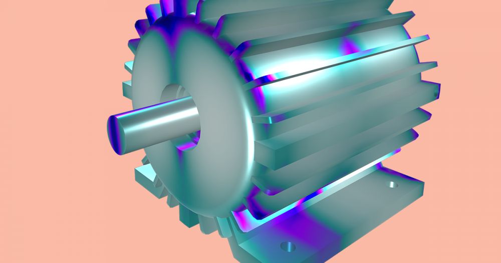
The iron and copper losses computed using the Loss Calculation subfeature can be coupled with the Heat Transfer (HT) interface to analyze the thermal performance. The Heat Transfer interface in COMSOL Multiphysics offers several ways to investigate the cooling of the machine. Natural or forced convection can be modeled either implicitly — by using a heat transfer coefficient from the outer surfaces — or explicitly, by modeling a laminar or turbulent fluid flow over the outer motor surfaces. A comparative study of the steady-state temperature can be done under different cooling conditions to determine the most appropriate cooling method for a particular motor application.


Temperature rise with natural air convection (left), forced air convection with a flow velocity of 1 m/s (center), and forced water cooling with a flow velocity of 50 mm/s (right).
The surface plots show the temperature in degrees for a rotor speed of 3000 rpm and stator current of 2 A. In this case, simply by inspection, we can determine that insulation class 180 (H) will be needed if natural convection is used. If forced convection is used, the insulation requirement will be reduced to class 130 (B) and with water cooling, class 105 (A) insulation will be sufficient. Here, we are assuming that the material of the permanent magnets has been appropriately selected considering thermal demagnetization effects.
Investigating the Efficiency of Electric Motors
In the end, the analysis of a motor design is about finding its efficiency. Efficiency tells us what fraction of the input power is obtained as mechanical output. The efficiency of a rotating machine varies with the generated electromagnetic torque and the rotor speed. Ideally, it is desirable to operate the machine at its maximum efficiency, but in practice, the torque-speed curve of the load driven by the motor will also have to be considered. As a consequence, the motor will be used in a certain operating range. The next best approach is to choose a motor that has the highest efficiency values in the operating regime.
This is where the efficiency map comes into the picture. The efficiency map of a motor is a plot of the efficiency against the variation in rotor speed and the electromagnetic torque. In other words, it can also be described as the plot of efficiency in the state-space of torque and speed. The load characteristic curve can be superimposed on the efficiency map to determine the overall efficiency of the system for the given load curve.
For instance, the load for electric vehicles is characterized by torque and speed drive cycles. The drive cycle consists of the load torque and speed variation with time. At each instant of time, a combination of torque and speed value specifies the load behavior. The scatter plot of all such torque–speed data points on the efficiency map helps to determine what overall efficiency is offered by the motor to a particular drive cycle. This enables the estimation of the total energy consumed by the motor during the complete drive cycle and subsequently predicting the range of the electric vehicle after a single charge.
COMSOL Multiphysics offers built-in modeling features that empower you to easily generate the efficiency map for your motor design. The Force Calculation feature gives you the electromagnetic torque. The Loss Calculation subfeature helps you get the iron and copper losses. The Heat Transfer interface can be used to compute the temperature rise due to losses, which can be fully coupled with the Rotating Machinery, Magnetic interface using the Multiphysics node to include the electromagnetic effects of the temperature rise. Finally, the Table Graph feature makes it possible to plot the efficiency map.


Analytically generated efficiency map using empirical coefficients (left) and an efficiency map obtained from a parametric simulation.
Here, all efficiency maps show the percentage efficiency. The first efficiency map has been generated analytically, as elaborated in the first section. The second efficiency map has been directly obtained from a parametric analysis. The horizontal line at the top of the plot shows that the maximum torque corresponds to a stator current of 5 A. The analytic and numeric efficiency maps show a reasonable agreement.


Efficiency map obtained from simulations including the effects of temperature rise (left) and a motor temperature map (right).
Unlike the first two efficiency maps, the third map includes the effect of temperature rise with natural air convection cooling. We can observe a reduction in the average rotor torque values for the same range of stator current values, after considering the effect of temperature rise. Furthermore, as the temperature increases at higher speeds (due to the increased losses), the torque reduces further because of a reduction in remanent flux in the rotor’s permanent magnets. This can be observed by following the line corresponding to “I = 5A” at the top of the plot. The net result is a change in efficiency distribution due to temperature rise. This helps to better evaluate the suitability of a given motor design for the application of interest. The temperature map shows the average stator temperature. It facilitates the determination of the required insulation class and the material of the permanent magnets by focusing on the relevant regime of motor operation.
Closing Remarks
We have briefly taken a look at the energy balance in the context of motor simulations. Such a power balance verification helps you to perform sanity checks on the results obtained from any FEM simulation tool.
Parametric analysis can be used to study the variation of electromagnetic torque as well as iron and copper losses with rotor speed and stator current. Such analyses can be used to extract the torque constant and empirical coefficients to estimate the losses at any speed and the current value for a given motor design.
We investigated the temperature rise due to losses in motors, which makes a major impact on the electromagnetic torque, the efficiency, and the required insulation class and material of the permanent magnets. A comparative study of the temperature rise under different cooling conditions makes it easy to choose a suitable cooling method.
Finally, we talked about the efficiency map, a crucial tool for determining whether a given motor design meets the needs of an application. Examining the efficiency map after considering temperature rise allows us to make a refined judgement on the machine’s performance in the context of an intended application.
Try It Yourself
Try computing the loss, temperature, and efficiency of an electric motor yourself. Access the MPH-file for the model discussed here by clicking the button below:

Comments (7)
maithem sabri
September 23, 2021excellent
Rahul Bhat
October 4, 2021Thank you Maithem for the prompt appreciation!
Nikki Musk
October 4, 2021this is really good article, thank you for sharing with us https://bit.ly/3BjzHvi
Regards, https://bit.ly/3Dkw1db
Rahul Bhat
October 4, 2021Thank you Nikki for the appreciation!
Amara Aymen
June 2, 2023Dear Rahul Bhat ,
I hope you are doing well. I have been thoroughly reviewing a reference model for temperature distribution in electrical motors and have a couple of questions that I believe your expertise can help answer.
1. In study 2, I noticed that the model was divided into four distinct steps. I am curious to understand the reasoning behind this division. Specifically, I would like to grasp how each step contributes to the overall temperature calculation process and how they interact with one another. Any insight you can provide on this matter would be greatly appreciated.
2. Additionally, while examining the reference model, I observed modifications made to the solver. I am particularly interested in understanding the specific changes that should be implemented for accurate temperature calculations. Could you please elaborate on the necessary modifications that I should consider making to the solver settings?
I highly value your professional expertise, and any guidance you can offer on these questions would be immensely helpful. Thank you in advance for your time and assistance.
Best regards,
Rahul Bhat
June 30, 2023Dear Amara,
Thank you for your response.
1. The steps are organized to first get the losses and use them to compute the temperature. The temperature is used to model the coil resistivity and remanent flux density of magnets at elevated temperature. Then the efficiency is computed with the updated losses. You can examine the slide #6 in the slidedeck available with the model file.
2. If you run a parametric sweep where the last study step is Time to frequency losses, then the Parametric solutions only save the solutions corresponding to last study step for all parameter values. The penultimate time dependent study solutions are not stored for all parameter values. Only the last solution is saved. Hence additional Solutions are added under the Job configurations>>Parametric sweep, for storing all the solutions corresponding to the intermediate study steps.
I hope that addressed your queries.
Best regards,
Quoc Thang Vo
October 4, 2023Dear Rahul Bhat ,
I would like to build an Efficiency Map for my Electrical Machine. Following thought your document, I didn’t see any control strategy (such as Maximum Torque Per Ampere (MTPA) control strategy or flux-weakening control strategy) considered in the model. It seems that there is no such control strategy built into COMSOL, so do you think that I would need to define the control outside of COMSOL, for example via LiveLink for Simulink or LiveLink for Matlab?
Please give me some hints or related materials if you have to calculate Efficiency Map with control strategy.
Best regards,