The latest version of the AC/DC Module enables you to create electrostatics models that combine wires, surfaces, and solids. The technology is known as the boundary element method and can be used on its own or in combination with finite-element-method-based modeling. In this blog post, let’s see how the new functionality can be used to conveniently set up a model that includes a number of very thin spiral wires.
Interfaces Based on the Boundary Element Method in COMSOL Multiphysics®
The boundary element method (BEM) is complementary to the finite element method (FEM) and is generally available in the COMSOL Multiphysics® software as of version 5.3. There are three different types of interfaces that are based on BEM, summarized in the table below:
| Interface | Applicable Physics | Products with Interface | Models Wires? |
|---|---|---|---|
| Electrostatics, Boundary Elements | Electrostatics in 2D and 3D | AC/DC Module | Yes |
| Current Distribution, Boundary Elements | Currents in electrochemical applications in 2D and 3D | Electrodeposition Module, Corrosion Module | Yes |
| PDE, Boundary Elements | Laplace’s equation in 2D and 3D | COMSOL Multiphysics (no add-on product required) | No |
These interfaces are quite similar. Although this blog post focuses on the interface for electrostatics, some of the techniques shown here are applicable if you are interested in the other two interfaces.
What Is the Boundary Element Method?
In contrast to FEM, BEM doesn’t require the generation of a robust volumetric mesh throughout your computational domain, which can be difficult and resource-intensive to achieve. BEM eliminates the problem by only requiring a surface mesh, which is significantly easier to generate. However, this advantage comes at a price. The COMSOL Multiphysics implementation of BEM cannot be used to model, for example, nonlinear or general inhomogeneous materials. The table below summarizes the pros and cons of BEM and FEM in the COMSOL Multiphysics implementation.
| Modeling Task | Using BEM | Using FEM |
|---|---|---|
| Infinite domains | Easy | Requires infinite elements or an approximation of an infinite domain through using large enclosing truncation domains |
| Postprocessing at arbitrary distances | Easy | Requires recomputing with a larger truncation domain |
| Wires | Easy, can be modeled with curves | Requires meshing the diameter of the wires to avoid mesh-dependent solutions |
| Volume mesh | Not required | Required |
| Isotropic materials | Easy | Easy |
| Anisotropic materials | Not available | Easy |
| Nonlinear materials | Not available | Easy |
By combining domains modeled with FEM and regions modeled with BEM, you can get the best of both worlds. For example, you can have one domain with an anisotropic material modeled with the traditional Electrostatics interface in the AC/DC Module and a surrounding isotropic domain modeled with the new Electrostatics, Boundary Elements interface.
Example: Electrostatic Precipitation Filter
To illustrate using the Electrostatics, Boundary Elements interface, let’s create a simplified model of an electrostatic precipitation filter. This type of filter is used in various industrial settings to filter particles from, for example, exhaust gases from coal power plants. An array of high-voltage wires creates a corona discharge region surrounding them, which in turn charges the unwanted particles. The charged particles then migrate in the electric field toward grounded metal plates (the collecting electrodes) and are periodically scraped off when the layer of particles becomes so thick that it deteriorates the performance of the filter.
Simulating the entire physical process of corona discharge, ionization, and charged particle migration is complicated and beyond the scope of this blog post. Instead, let’s look at the filter from a purely electrostatics perspective. This keeps the model simple, yet quite general, and illustrates a modeling approach that is applicable to a wide range of other electrical devices. If you want to know more about the details of modeling an electrostatic precipitation filter, see page 21 of COMSOL News 2012.
The filter in this example consists of 6 ground plates and 60 wires, as shown in the figure below. The wires are modeled as parametric curves and held at 50 kV.
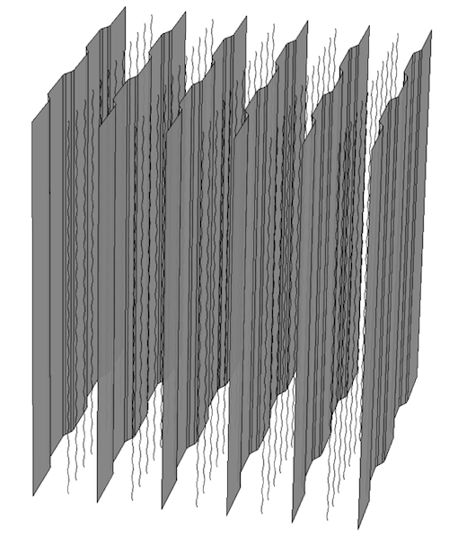
The electrostatic precipitation filter example.
Assigning Material Properties
In the real case, this filter would be held in a frame, which we have neglected here to keep things simple. We assume that the space between and outside the plates is filled with air, which is the only material property in this model. In this example, we study this component as “hanging in midair” to get its idealized electrostatics properties. To assign air to the model, notice that there is no domain to click. Instead, you select the air region surrounding the model by selecting All voids from the selection list in the Settings window for the Air material. The only available void in this example is called the Infinite void and represents the region between the plates all the way “out to infinity”, as shown below.
For more information on the difference between solid domains and voids, see the Release Highlights page.

The settings for the Air material.
Selecting the Infinite void in this way is all that has to be done to model an infinite region when using boundary elements. Had we modeled this with FEM, then we would have needed to enclose the geometry model in a finite-sized box (or some other shape). To increase the accuracy of the computation, we would have also needed to add extra layers with Infinite Element domains surrounding the box.
Applying Boundary Conditions
The boundary conditions are set at two levels: for boundary surfaces and for edges. The figure below shows the Ground boundary condition assigned to the ground plates.

The settings for the Ground boundary condition.
There is a more interesting condition on the wires. They are assigned a Terminal edge condition with the Terminal type set to Voltage at 50 kV. In addition, the Edge radius is set to 1 mm, as shown in the figure below.

The settings for the Terminal edge condition.
Notice how the radii of the wires are entered into the model on the physics side and not on the CAD side. The CAD model of the wires consists of parameterized curves that have no radial extent but are (mathematically speaking) one-dimensional objects. This modeling approach shows a major benefit of BEM. If the model had been set up with the finite-element-based interface for electrostatics, then the wires would have to be modeled as thin spiral-shaped tubes with a finite-sized radius, thereby generating a mesh with many elements. Although possible, BEM is much more convenient.
Solvers for the Boundary Element Method
FEM produces large sparse matrices, whereas BEM generates large filled matrices. This calls for solvers specialized in manipulating such. As a matter of fact, the system matrix produced by BEM is so heavy to handle that it cannot even be formed in its entirety. Instead, only those parts of the matrix that are needed by the solver for the moment are generated. More specifically, only the matrix-vector multiplications needed for the moment are performed. The method implemented in COMSOL Multiphysics for fast matrix-vector multiplications is called the adaptive cross approximation method and is used automatically when you are using one of the BEM interfaces. If you are interested, you can read more about the related solver options for version 5.3.
On one hand, BEM requires fewer degrees of freedom in order to produce accurate results as compared with FEM. On the other hand, BEM is more computationally demanding, so in the end, the methods are comparable with regard to computational demand versus accuracy.
Postprocessing and Visualization
For finite-element-based models, the computed fields in the modeled volume are visualized using slice plots, isosurface plots, arrow plots, flux lines, etc., by means of the volumetric finite element mesh. When using BEM, there is no volumetric mesh available, so in order to visualize spatially varying fields, a regular grid is used as a substitute. The regular grid is defined as a Grid 3D data set and lets you define a rectangular box with maximum and minimum values of its extents in the x, y, and z directions. In addition, the x-, y-, and z-resolution settings correspond to the element size and determine the granularity of the visualization. In the figure below, the resolution is set to 100 by 200 by 200, which corresponds to 4 million hexahedral grid elements.
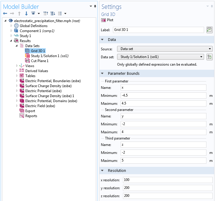
The settings for the Grid 3D data set.
Boundary element fields can be quite heavy to postprocess and visualize and it can be a good idea to turn off Automatic update of plots. The corresponding check box is available in the Settings window for the Results node, as shown below.
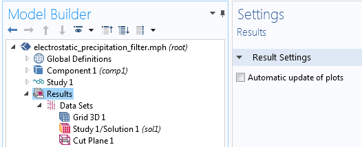
The check box for Automatic update of plots in the Result node settings.
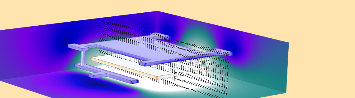
The visualization below shows the electric potential field around the wires, between the plates, and surrounding the plates. By increasing the size of the Grid 3D box, you can extend the visualization to a larger volume without having to recompute the solution. This is another benefit of BEM, since with FEM, you would need to enlarge the truncation domain and recompute.
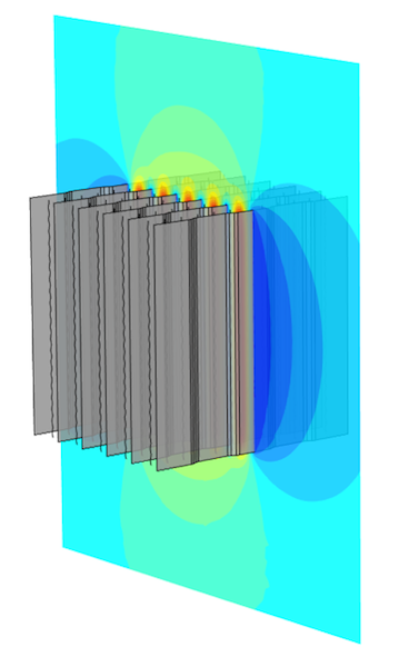
The electric potential field for the electrostatic precipitation filter example.
Models with Multiple Dielectric Materials
A limitation with BEM is that each modeling domain is required to have a constant and isotropic material property. In the case of electrostatics, each domain must have a constant permittivity. You can create models with several domains of different permittivity values. The figure below shows a MEMS capacitor model with two permittivity values:
- Air in the exterior infinite void
- Dielectric material between the two electrode plates
To make this type of model possible, each distinct dielectric domain needs to have its own Charge Conservation node added under the Electrostatics, Boundary Elements interface. Within each Charge Conservation domain, or group of domains, the permittivity is a constant. The capacitance of this type of device is computed using the predefined variable for capacitance under Derived Values, just like the corresponding finite-element-based model would.

A MEMS capacitor model example with multiple permittivity values.
Hybrid Finite Element and Boundary Element Modeling
COMSOL Multiphysics version 5.3 comes with a predefined multiphysics coupling that combines finite-element-based and boundary-element-based electrostatics. The figures below show another version of the MEMS capacitor model, where the dielectric material is replaced by an anisotropic piezoelectric material (PZT-5H). Since the Electrostatics, Boundary Element interface doesn’t allow for simulating anisotropic materials, the traditional finite-element-based Electrostatics interface is used in that region.
In addition, a small box surrounding the capacitor is also modeled using the finite-element-based interface. In this example, the Electrostatics, Boundary Elements interface is only active in the exterior infinite void. The coupling between the finite element region and boundary element region is defined under the Multiphysics node in the settings for Boundary Electric Potential Coupling.

The settings to combine finite-element-based and boundary-element-based electrostatics.
The figure below shows the electric potential visualized in both the finite element and boundary element regions. Some numerical artifacts due to interpolation can be seen in the junction between the finite element and boundary element domains. Such artifacts vanish when computing using a finer mesh and visualizing using a higher resolution for the Grid 3D data set.

The electric potential field for the MEMS capacitor model example.
Try It Yourself
You can download the example models highlighted in this blog post by clicking the button below.
Two other boundary-element-based electrostatics tutorials are available in the Application Gallery:
- MEMS capacitor with a single dielectric domain
- Capacitive position sensor
The capacitive position sensor demonstrates the use of the Electrostatics, Boundary Elements interface in combination with a Deformed Geometry interface for modeling large geometrical displacements. In addition, the same model demonstrates using the accelerated capacitance-matrix-calculation option Stationary Source Sweep, which is new in version 5.3 of COMSOL Multiphysics. The Stationary Source Sweep study type can also be used with the finite-element-based Electrostatics interface.


Comments (3)
Boris Narozhny
October 6, 2017Thank you for the informative post. However, the examples you discuss are fairly complex. At the same time, I can find little or no guidance on how to use COMSOL to reproduce known solution of textbook problems. As a physicist, I find that solving simple problems is extremely useful before tackling more complicated ones.
The problem I have trouble with is the simple enough problem of the electric potential created by the non-uniform 2D charge density. In this case, the Poisson equation contains a delta-function in the right-hand side which can be interpreted as a boundary condition to the Laplace equation. It is setting this boundary condition in COMSOL that puzzles me at the moment. So, what do I need to do in order to solve the 3D Laplace equation with the boundary condition on a flat 2D surface, which is “mixed”, i.e. contains both the potential and its derivative?
Magnus Olsson
October 9, 2017Dear Boris,
Can you explain more exatly what you want to model? Prescribing both the electric potential and the eletric field can easily result in an unphysical and/or ill-posed model. Thus, there are no general ways of doing that in a finite element model. The most common mixed boundary condition is the so called Robin condition that can be used to model a thin electrode held at potential “V1”, that is coated with a thin dielectric film. That is:
nD = (V1-V)*epsilon/d
where “nD” is the normal electric displacement field and V is the electric potential on the surface of the thin dielectric layer with permittivity “epsilon” and thickness “d”. Note that “V1” and all other parameters may be functions of the spatial coordinates and of the solution (V) and its spatial derivatives.
Here the normal field is prescribed as the result of an applied potential “V1” and a physical mechanism (capacitive layer) that yields a well-posed model.
Other physics effects may require the addition of extra equations and state variables to implement in a sound way.
Best regards,
Magnus
Boris Narozhny
October 12, 2017Dear Magnus,
I want to solve the Laplace equation to find the electric potential created by a non-uniform charge density that is located on a finite-size 2D surface, say a rectangle. A physical example to this is the inhomogeneous electric current flow in a 2D conductor. This effect can be completely described by the Laplace equation in 3D, namely in the half-space above the plane of the rectangle and the boundary condition which specifies the z-derivative of the potential being given by the potential itself plus some function of the coordinates (z direction is normal to the rectangle). If the rectangle is “infinite” in say x direction, then the problem can be further simplified, since in that case all quantities in the plane will be functions of y only. But, if the rectangle is finite, then there is non-trivial dependence on both x and y. The resulting potential in 3D space will also be strongly asymmetric.
Best regards,
Boris.