

In a previous blog post, we discussed integration methods in time and space, touching on how to compute antiderivatives using integration coupling operators. Today, we’ll expand on that idea and show you how to analyze spatial integrals over variable limits, whether they are prescribed explicitly or defined implicitly. The technique that we will describe can be helpful for analyzing results as well as for solving integral and integro-differential equations in the COMSOL Multiphysics® software.
Variable Limits of Integration
In COMSOL Multiphysics, we can evaluate spatial integrals by using either integration component coupling operators or the integration tools under Derived Values in the Results section. While these integrals are always evaluated over a fixed region, we will sometimes want to vary the limits of integration and obtain results with respect to the new limits.
In a 1D problem, for example, the integration operators will normally calculate something like
where a and b are fixed-end points of a domain.
What we want to do instead, though, is to compute
and obtain the result with respect to the variable limit of integration s.
Since the integration operators work over a fixed domain, let’s think about how to use them to obtain integrals over varying limits. The trick is to change the integrand by multiplying it by a function that is equal to one within the limits of integration and zero outside of the limits. That is, we define a kernel function
\begin{cases}
1 \quad x \leq s\\
0 \quad \mathrm{otherwise},
\end{cases}
and compute
As indicated in our previous blog post about integration methods in time and space, we can build this kernel function by using a logical expression or a step function.
We also need to know how the auxiliary variable s is specified in COMSOL Multiphysics. This is where the dest operator comes into play. The dest operator forces its argument to be evaluated on the destination point rather than on the source points. In our case, if we define the left-hand side of the above equation as a variable in the COMSOL software, we type dest(x) instead of s on the right-hand side.
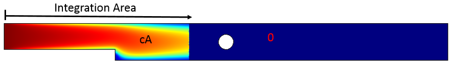
Let’s demonstrate this with an example. In this case, a model simulates a steady-state exothermic reaction in a parallel plate reactor. There is a heating cylinder near the center and an inlet on the left, at x = 0. One of the compounds has a concentration cA.
What we want to do is to calculate the total moles per unit thickness between the inlet and a cross section at a distance of s from the inlet. We then plot the result with respect to the distance from the inlet.
First, we define an integration coupling operator for the whole domain, keeping the default integration operator name as intop1. If we evaluate intop1(cA), we get the integral for the entire domain. To vary the limit of integration horizontally, we build a kernel using a step function, which we’ll call step1. We then define a new variable, intUpTox.


Combining the integration coupling operator, dest operator, and new variable to evaluate an integral with moving limits.
Let’s see how the variable described in the image above works. As a variable, it is a distributed quantity and has a value equal to what the integration operator returns. During the integration, we evaluate x at every point in the domain of integration and dest(x) only at the point where intUpTox is computed. We find a horizontal line that spans from the inlet all the way to the outlet and plot intUpTox.

Integrating concentration cA over a horizontally varying limit of integration.
If we instead plot intUpTox/intop1(cA)*100, we get a graph of the percentile mass to the left of a given point with respect to the x-coordinate.
In the above integral, the limit of integration is given explicitly in terms of the x-coordinate. Sometimes, though, the limit may only be given in an implicit criteria, and it may not be straightforward to invert such criteria and obtain explicit limits. For example, say that we want to know the percentage of total moles within a certain radial distance from the center of the heating cylinder. Given a distance s from the center (xpos, ypos) of the cylinder, we want a kernel function equal to one inside the radial distance and zero outside of it. To do so, we can use:
But how do we specify s? We again use the dest operator: s^2 = (\mathrm{dest}(x)-x_{pos})^2+(\mathrm{dest}(y)-y_{pos})^2, and the kernel is

We implement this method by defining a Cut Line data set to obtain the horizontal line through the hole’s center and placing a graph of our integration expression over it. It is not necessary that the cut line is horizontal; it just needs to traverse the full domain that the integration operator defines. Furthermore, s should vary monotonically over the cut line.

New data set made with a cut line passing through the center of the hole.
In the image below, we added an insert by zooming in at the bottom left area of the graph. This section shows that there is no result on the plot for a distance of less than 2 mm from the center of the heating hole. This is because that region is not in our computational domain. Since the hole has a radius of 2 mm, the ordinate starts at 0 at an abscissa of 2 mm.

Percentage of mass in a domain, which is within a radial distance from the fixed point. The radial distance is varied by using the dest operator in an implicit expression.
Integral and Integro-Differential Equations
In the previous sections, we evaluated integrals where the integrands were given. But what do we do if we have the integral and want to solve for the integrands? An example of such a problem is the Fredholm equation of the first kind
where we want to solve for the function u when given the function g and Kernel K. These types of integral equations often arise in inverse problems.
In integro-differential equations, both the integrals and derivatives of the unknown function are involved. For example, say we have
and want to solve for u given all of the other functions.
In our Application Gallery, we have the following integro-partial differential equation:
where we solve for temperature T(x) and are given all of the other functions and parameters.
We can solve the above problem using the Heat Transfer in Solids interface. In this interface, we add the right-hand side of the above equation as a temperature-dependent heat source. The first source term is straightforward, but we need to add the integral in the second term using an integration coupling operator and the dest operator. For the integration operator named intop1, we can evaluate
with intop1(k(dest(x),x)*T^4).
For more details on the implementation and physical background of this problem, you can download the integro-partial differential program tutorial model here. Please note that some integral equations tend to be singular and we need to use regularization to obtain solutions.
Summary of Spatial Integration Over Varying Limits
In today’s blog post, we’ve learned how to integrate over varying spatial limits. This is necessary for evaluating integrals in postprocessing or formulating integral and integro-differential equations. For more information, you can browse related content on the COMSOL Blog:
- Overview of Integration Methods in Space and Time
- How to Integrate Functions Without Knowing the Limits of the Integral
- Analyze Your Simulation Results with Projection Operators
For a complete list of integration and other operators, please refer to the COMSOL Reference Manual.
If you have questions about the technique discussed here or with your COMSOL Multiphysics model, feel free to contact us.


Comments (0)