

The dynamics of magnetization in magnets are described by micromagnetic theory, governed by the Landu–Lifshitz–Gilbert equations. We built a customized “Micromagnetics Module” using the Physics Builder in the COMSOL Multiphysics® software, which can be used to perform micromagnetic simulations within the framework of the COMSOL® software. This Micromagnetics Module can be coupled straightforwardly to other add-on modules to perform multiphysics micromagnetic simulations, such as magneto-dipolar coupling, magneto-elastic coupling, magnet-thermal coupling, and more. The module package, along with a user’s guide, is available for download.
Introduction to Magnonics and Micromagnetics
Magnonics is a subfield of spintronics or magnetism (Ref. 1). It is similar to its counterparts, phononics and photonics, but focuses on energy and information transport carried by spin waves (or magnons in the quantum limit), which are elementary excitations of magnetic systems. Spin waves can carry energy, linear and angular momentum, as well as information. Magnetic insulators such as YIG (Y3Fe5O12), because of its extremely small damping and absence of Joule heating (Ref. 2), are ideal materials for spin wave manipulation. Furthermore, spin waves can interact with magnetic textures (Ref. 3), such as magnetic domain walls, vortexes, and skyrmions — thereby offering a new route for operating magnetic memories. This makes magnonics a promising candidate for the next generation of information technology.
In this blog post, we will demonstrate how to use the Micromagnetics Module to perform numerical micromagnetic simulations of spin wave dynamics in COMSOL Multiphysics.
Micromagnetic Modeling Theory
The dynamics of magnetic moments in magnetic materials is governed by the Landau–Lifshitz–Gilbert (LLG) equation. The spirit of micromagnetic modeling is to treat all magnetic moments in one or several unit cells as one semiclassical macrospin, which is denoted by a unit vector \textbf{m} defined as
where \textbf{M}(\textbf{r}, t) is the temporal-spatial distribution function of total magnetization and M_s is the saturation magnetization of the material.
The time evolution of this unit moment vector follows the LLG equation (Ref. 4)
where the dot indicates the time derivative, \gamma is the gyromagnetic ratio, \alpha is the Gilbert damping coefficient, and H_{\rm{eff}} is the effective field exerted on the local moment, which is defined as
with \mu_0 as the vacuum permeability and Ethe free energy of the magnetic system, including all possible interactions.
Let’s assume the simplest case: one macrospin in a static magnetic field applied along the z direction. The effective field is simply H_{\rm{eff}}=H \hat{e}_z. Starting from the initial state with the macrospin slightly tilted away from the equilibrium z direction, the macrospin vector then precesses around the effective field in a right-handed fashion according to the LLG equation. In the presence of Gilbert damping (the term with \alpha), the kinetic energy of the system is finally dissipated and the macrospin relaxes to its energy minimum, i.e., aligned with the effective field. Such precessing dynamics are related to ferromagnetic resonance (FMR), where the angular frequency depends linearly on the strength of the applied field.
Spin waves appear when introducing nonlocal interactions, e.g., short-ranged exchange interactions that take the following form in the continuum limit H_{\rm{eff}}=A \triangledown^2\textbf{m}, with A the exchange stiffness coefficient. In the presence of the exchange interaction, the precessing mode of a single macrospin can transport to neighboring macrospins, resulting in a propagating angular momentum current, e.g., spin waves.
Electromagnetic and elastic waves can be confined or steered via a nanostructure design, and so can spin waves. Furthermore, spin waves can be manipulated by magnetic textures, the inhomogeneous distribution of the magnetization order. One example is the magnetic domain wall, the transition region between two magnetic domains with opposite magnetization. It’s shown both theoretically and experimentally that the domain wall can serve as a conducting channel for spin waves, which can be used to design reconfigurable spin wave circuits.
Micromagnetic simulations can provide assistance to explain experimental findings. There have also been many successful examples that micromagnetic simulation can predict novel phenomena, which are then verified by experiments.
The Micromagnetics Module Developed by the Physics Builder
There are two popular open-source micromagnetic simulation software: Object Oriented MicroMagnetic Framework (OOMMF) and GPU-accelerated Mumax3.
There are two reasons we prefer to perform micromagnetic simulation using COMSOL Multiphysics instead:
- COMSOL Multiphysics is based on the finite element method, rather than the finite difference method used by OOMMF and Mumax3. The finite element method becomes more powerful when modeling complex geometries and structures.
- The Micromagnetics Module can be used directly with the rich physics modules within COMSOL Multiphysics. For instance, by combining the AC/DC Module (electric currents and electromagnetic fields) and RF Module (microwaves), we can model the dipolar interaction in a magnet. Combining the custom-built module with the Structural Mechanics Module, you can model magneto-elastic effects, and the Heat Transfer Module can be used to model thermal effects in a magnet. Multiphysics couplings between the customized physics and add-on products becomes straightforward within this framework.
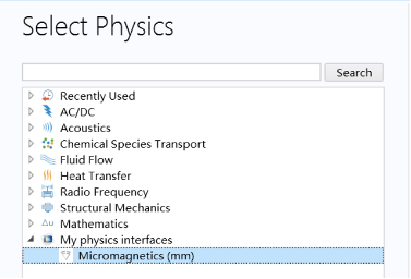
Users who are interested in using the Micromagnetics Module for COMSOL Multiphysics can install the compiled module file, Micromagnetics Module.jar, to local COMSOL archives. A new physics interface, Micromagnetics (mm), appears when selecting physics.
The Micromagnetics Module (V1.33) has the user interface shown below.
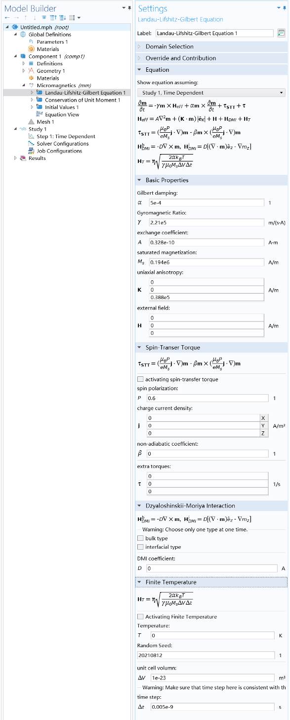
The Micromagnetics Module (V1.33) has almost all features presented by other open-source software, including but not limited to:
- Basic Landau–Lifshitz–Gilbert formalism, including exchange interactions and uniaxial anisotropy
- Dzyaloshinskii–Moriya interaction (both bulk and interfacial types) with appropriate boundary conditions
- Spin-transfer torque with both damping- and field-like terms
- Arbitrary field and torque input (time- and space dependent)
- Finite temperature effect (with arbitrary random seed)
- Pinning boundary conditions and periodic boundary conditions
- Capability of solving multiple independent LLG equations in one region (such as synthetic antiferromagnets with multiple sublattices)
- Capability of multiphysics coupling, including magneto-dipolar coupling, magneto-elastic coupling, magneto-electric coupling, and magneto-thermal coupling
Based on the Micromagnetics Module, we have demonstrated many interesting spin wave physics and proposed various spin wave devices, such as the spin-wave diode (Ref. 5), spin-wave fiber (Ref. 6), spin-wave polarizer and retarder (Refs. 7–8), and magnetic logic gates (Ref. 9).
Multiphysics Couplings with the Micromagnetics Module
As mentioned above, one advantage of COMSOL Multiphysics is the capability for multiphysics couplings between the add-on modules. Spin waves can be manipulated by magnetic fields, lattice deformations, temperature gradients, etc. Coupled systems of spin waves and other excitations (such as electromagnetic and elastic waves) can combine the advantages of both worlds and produce rich physics, facilitating information generation and transmission. Now we will demonstrate what multiphysics couplings can be done based on the Micromagnetics Module.
Cavity magnonics (Ref. 10) is the interdiscipline of magnonics and cavity quantum electrodynamics (CQED). One of the applications of CQED is to realize quantum information processing by manipulating photon–matter interaction. A typical configuration in cavity magnonics is a microwave cavity with magnets placed inside. The magnets are coupled to the standing or propagating electromagnetic waves in the cavity. Such systems offer a new option to study the manipulation of spin current and nonlinear dynamics of magnetic moments (Refs. 11–12). The cavity magnonic system can be simulated by coupling the Micromagnetics Module and RF Module. For magnetostatic simulation, coupling between the Micromagnetics Module and AC/DC Module (magnetic fields) is sufficient.
Spin mechanics includes the interaction between magnetization and lattice deformation. In materials with magneto-elastic coupling (or magnetostriction), the spatial and temporal changes of magnetization (spin waves) exert forces on the lattice, and the deformed lattice (elastic waves) produces fields acting back onto the magnetization. For example, as the animation below shows, a magnetized disk is excited by magnetic fields, and the precessing magnetization radiates elastic waves to the substrate. The spin-mechanical problem can be simulated by coupling the Micromagnetics Module and Solid Mechanics Module.
Self-Adaptive Textures with Electric Current
In metallic magnets, spin-polarized electric currents exert spin-transfer torque to local magnetic moments, causing current-driven texture motion. Since the conductivity within magnetic film depends on the relative orientation of local magnetization and current direction due to the anisotropic magnetoresistance (AMR), the interplay between the current, torque, and texture can be modeled using the Micromagnetics Module with the AC/DC Module (electric currents).
As the animation below shows, the voltages applied on two electrodes modify the magnetic textures (top) via spin-transfer torque. Consequently, the local conductivity and the current density distribution (bottom) change accordingly. The magnetic textures finally adapt to a stable configuration, leading to an increasing conductance between two electrodes. It’s proposed that such a positive feedback behavior can be used for neuromorphic computing (Ref. 13).
How to Access the Micromagnetics Module
We distribute the Micromagnetics Module file freely via:
The downloaded package includes the module installation file and a user’s guide with installation instructions and examples. We appreciate any suggestions, reports, and communication from users. More features will be updated actively in future versions.
Acknowledgement
The author acknowledges the supervision of Prof. Jiang Xiao at Fudan University and the support from the Institute for Nanoelectronic Devices and Quantum Computing at Fudan University.
About the Author
Dr. Weichao Yu has a BS in applied physics from the School of Physical Science and Engineering, Tongji University, China, and a PhD in theoretical physics from Fudan University, China. He worked as a postdoctoral researcher at Fudan University and an assistant professor at the Institute for Materials Research, Tohoku University, Japan. He is currently a researcher at the Institute for Nanoelectronic Devices and Quantum Computing at Fudan University. Yu’s research interests include theoretical research on fundamental phenomena in spintronics and magnetism, including the dynamics of magnetic textures and spin waves and coupling between magnetic systems with other multiphysics systems, such as spin cavitronics or cavity spintronics (coupling between magnon and photon) and spin mechanics (coupling between spin waves and elastic waves). He proposes and designs new types of spintronic devices and new concepts for unconventional computing, such as logic-in-memory computing based on magnetic systems and neuromorphic computing with self-learning features. He has also developed a micromagnetic simulation module based on the finite element method with the capability of bidirectional coupling with other multiphysics systems, facilitating the study of fundamental magnetism and the design of new spintronic devices.
References
- A. Barman et al., The 2021 Magnonics Roadmap, J. Phys.: Condens. Matter, vol. 33, no. 413001, 2021.
- A. V. Chumak et al., Magnon Spintronics, Nature Physics, vol. 11, no. 453, 2015.
- H. Yu, J. Xiao, and H. Schultheiss, Magnetic Texture Based Magnonics, Physics Reports, vol. 905, no. 1, 2021.
- V. G. Bar’yakhtar and B. A. Ivanov, The Landau-Lifshitz Equation: 80 Years of History, Advances, and Prospects, Low Temperature Physics, vol. 41, no. 663, 2015.
- J. Lan, W. Yu, R. Wu, and J. Xiao, Spin-Wave Diode, Phys. Rev. X, vol. 5, no. 041049, 2015.
- W. Yu, J. Lan, R. Wu, and J. Xiao, Magnetic Snell’s Law and Spin-Wave Fiber with Dzyaloshinskii-Moriya Interaction, Phys. Rev. B, vol. 94, no. 140410, 2016.
- J. Lan, W. Yu, and J. Xiao, Antiferromagnetic Domain Wall as Spin Wave Polarizer and Retarder, Nature Communications, vol. 8, no. 178, 2017.
- W. Yu, J. Lan, and J. Xiao, Polarization-Selective Spin Wave Driven Domain-Wall Motion in Antiferromagnets, Phys. Rev. B, vol. 98, no. 144422, 2018.
- W. Yu, J. Lan, and J. Xiao, Magnetic Logic Gate Based on Polarized Spin Waves, Phys. Rev. Applied, vol. 13, no. 024055, 2020.
- B. Z. Rameshti, S. V. Kusminskiy, J. A. Haigh, K. Usami, D. Lachance-Quirion, Y. Nakamura, C.-M. Hu, H. X. Tang, G. E. W. Bauer, and Y. M. Blanter, Cavity Magnonics, ArXiv:2106.09312 [Cond-Mat], 2021.
- W. Yu, J. Wang, H. Y. Yuan, and J. Xiao, Prediction of Attractive Level Crossing via a Dissipative Mode, Phys. Rev. Lett., vol. 123, no. 227201, 2019.
- W. Yu, T. Yu, and G. E. W. Bauer, Circulating Cavity Magnon Polaritons, Phys. Rev. B, vol. 102, no. 064416, 2020.
- W. Yu, J. Xiao, and G. E. W. Bauer, A Hopfield Neural Network in Magnetic Films with Natural Learning, ArXiv:2101.03016 [Cond-Mat], 2021.

Comments (15)
Mohammad Qaid
January 25, 2022Hello,
Is there anyone who faced problems installing this module with v5.4, because I could not, it showed an error ” failed to initialize the physics interface”..
Thanks
伟超 余
January 25, 2022Hi Mohammad, thanks for leaving message. The module was developed by COMSOL 5.6. So it can be run at least by the 5.6 and versions later. Please update your software to 5.6 and try again.
Abdullah Al Maruf
June 2, 2022.
Yonatan Calahorra
August 4, 2022Looks very interesting I intend to try it in the next few weeks – thank you!
Harshitha Govindaraju
September 28, 2022Hello,
Do you have an example file where you have implemented this module for a given geometry and analyzed or plotted the results? Appreciate your valuable time. Great work!
Regards,
Harshitha Govindaraju
Rajesh Pathak
April 3, 2023I have attached micromagnetic module v2.2 with COMSOL 5.5 but its physics is not working. Please help
伟超 余
June 1, 2023As was stated in the manual, the module file was created by COMSOL V5.6, so you can only use it with version later than V5.6
Amin Pishehvar
June 1, 2023Hello,
I’m trying to replicate the results of Magnetostatic Coupling (AC/DC Module) of the micromagnetics module user’s guide and I follow the tutorial video precisely but I receive the message
Failed to find consistent initial values.
Last time step is not converged.
every time I run the simulation. Is there anything missing in the video or anything that must be mentioned and wasn’t? I also want to simulate spin cavitronics and I face the same error message. Is there a chance you could share the files for these simulations?
伟超 余
June 1, 2023As you can see in the video, I have shown every steps and all details. Pay special attention to unit of geometry, it’s supposed to [nm] rather than [m], which is by defaut and is always ignored. You can also try different combination of solver setup by refering to COMSOL refenrence manual.
I used to share mph files via Application Exchange page, but the room is too small so that I cannot share them anymore.
Guillermo Gestoso Carbajo
June 6, 2023Is it possible to obtain those .mph examples in a different way?
Ioannis C
January 17, 2024Hello,
Could you please share the link for the tutorial video you refer to?
Md Majibul Haque Babu
October 20, 2023Hello
I was trying to download it. Unfortunately, I didn’t. Can you tell me how can I download it?
Ilyasova Galiya
January 25, 2024Hello,
When creating a model in the Comsol Multiphysics 6.0 micromagnetic module, I had questions about the units of measurement of some quantities.
1. Your uniaxial anisotropy constant K is measured in [A/m].
2. Your exchange interaction constant A is measured in [A*m], in the micromagnetic module
At the same time, in the micromagnetic modeling software package Object Oriented MicroMagnetic Framework (OOMMF), the unit of measurement of uniaxial anisotropy constants K is specified [J/m3] and the unit of measurement of exchange interaction constants A is measured in [J/m].
Please explain how you obtained these units of measurement (perhaps you have given values).
Ilyasova Galiya
January 25, 2024Hello,
When creating a model in the Comsol Multiphysics 6.0 micromagnetic module, I had questions about the units of measurement of some quantities.
1. Your uniaxial anisotropy constant K is measured in [A/m].
2. Your exchange interaction constant A is measured in [A*m], in the micromagnetic module
Please explain how you obtained these units of measurement (perhaps you have given values).
Esther Du
February 1, 2024 COMSOL EmployeeHello,
Any question on this blog content you are welcomed to communicate with the author, Dr. Yu, by wcyu@fudan.edu.cn.