
Solution Joining for Parametric, Eigenfrequency, and Time-Dependent Problems

In a previous blog entry, we discussed the join feature in COMSOL Multiphysics in the context of stationary problems. Here, we will address parametric, eigenfrequency, frequency domain, and time-dependent problems. Additionally, we will compare and contrast the built-in with and at operators versus solution joining.
Joining Parametric Stationary Solutions
Consider a situation where you have solved a problem for a range of parameters using the Parametric Sweep feature in COMSOL Multiphysics and want to compare the results for the different values of the parameter against each other or a benchmark value of the parameter. An important example of this is a mesh convergence study, where the element size is the sweep parameter and the solution for each mesh size is compared with the solution on the finest mesh.
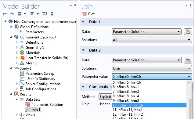
To evaluate the difference in some norm, you first need to make a join data set. As discussed earlier, when “joining”, or comparing, solutions, you will be asked to choose which two base data sets you intend to join: data1 and data2. For a parametric study, each base data set contains more than one solution. Thus, you have to decide whether you want to compare just one or all of your parameter values to the benchmark solution. In a mesh refinement study, for example, you can choose “All” for data1 and “One” for data2. When you choose “One”, COMSOL Multiphysics will present you with a drop-down menu, where you can pick the benchmark value.
In the figure below, the value of the element size parameter, hn, for the finest mesh is 16.
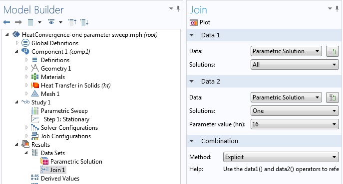
Joining a parametric solution comparing all of the parameter solutions to the benchmark solution from the finest mesh.
Once you have built the join data set, the next step is to use it in postprocessing. For the above 2D steady state heat transfer problem, consider the integral of the square of the difference in temperature, i.e., the L2-norm of the difference. To perform a spatial integration, go to Results in the Model Tree, right-click “Derived Values” and choose “Surface Integration” to get the following settings window:
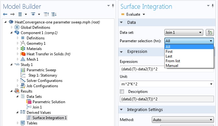
Settings window for calculating the the L2-norm of the difference in temperature .
Above, you can see that you have a choice of using one, some, or all of the parametric values for the postprocessing step. Note that this is possible because the “All” option was used for the first data set when you built the join data set. By choosing “All” in the Surface Integration settings window, when you then click “Evaluate”, the L2 difference between the solution on the finest mesh and all other meshes will be evaluated and tabulated. To this end, the COMSOL software takes the solution for each value of the sweep parameter and uses it for data1, whereas the solution for hn = 16 is used for data2. Using the Table Graph feature, you can obtain a plot of the difference versus the mesh size.
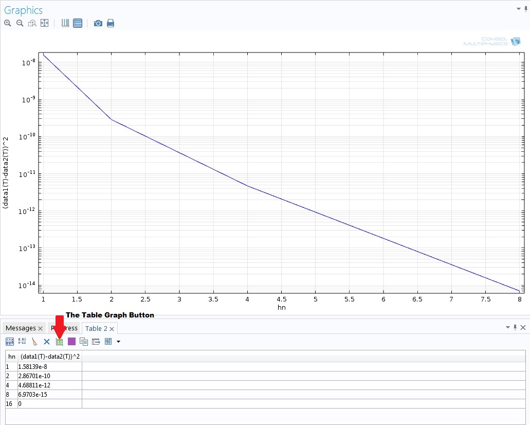
Plot using the specified join data set that compares the L2-norm of the difference in temperature versus the mesh size. The plot can be instantly made by using the Table Graph button.
Multiparameter Sweep
COMSOL Multiphysics allows you to perform parametric sweeps using more than one parameter. In a multiparameter sweep, you have two options for Sweep type: “All combinations” and “Specified combinations”. In the first case, the COMSOL software carries out a nested parametric sweep, where every combination of parameters is utilized. In the second case, a combination of parameter values with the same indices is constructed, where the parameter value lists for all parameters need to have the same lengths. As far as solution joining is concerned, this case is the same as a single parameter sweep. Thus, in the investigated case here, we will assume that the Sweep type is set to “All combinations”, where the parameter lists do not need to be of the same length.
In the mesh convergence study above, a convective heat flux boundary condition with heat transfer coefficient of 5 W/(m2K) was used as a boundary condition. Let us parameterize this coefficient, using the parameter name hflux, so as to compute the solution for all combinations of the heat transfer coefficient and mesh size. Here’s what that looks like:
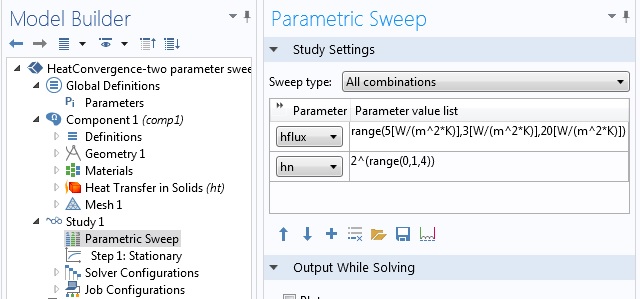
Setting up a multiparameter sweep. The heat transfer coefficient is parameterized from 5 W/(m2K) to 20 W/(m2K) with steps of 3 W/(m2K), while the mesh is parameterized in the same way as the previous case.
When you create the join data set, COMSOL Multiphysics gives you a vectorized list of the parameters in order to identify the base or benchmark solution. In this example, we should choose one of the combinations with hn = 16, which in our case will be hflux = 8 W/(m2K):
Join data set with a multiparameter sweep. The case for the finest mesh (hn = 16) and a heat transfer coefficient of 8 W/(m2K) is used as the benchmarking solution.
Finally, to evaluate the L2 norm difference, we use the Surface Integration like in the case of a single parameter sweep. The difference here is that instead of using all solutions, we only use the case with hflux = 8 W/(m2K) and all values of the mesh size. There can be reasons where all combinations have to be considered, but for a mesh refinement study, solutions with the same problem parameters (material properties, boundary conditions, etc.) require that only different mesh sizes are compared.
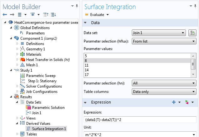
Specifying the L2 norm of the temperature difference for all mesh refinement parameters at a heat transfer coefficient value of 8 W/(m2K).
To repeat the convergence study for the next value of the heat transfer coefficient (11 W/(m2K)), you can go back to the Join settings window and choose the parameter combination for that value of hflux and hn = 16 as the second base solution.
Solutions on Different Domains
Sometimes, you may have base solutions defined on different domains. This can, for example, arise if a parameter used during geometry creation is applied in a parametric sweep. In such cases, the software implements the join data set only over the intersection of the domains used for the base solutions.
Eigenfrequency, Frequency Domain, and Time-Dependent Studies
The methods for stationary parametric studies as described above work similarly for other study types. For eigenfrequency, frequency domain, and time-dependent studies, the parameter sets will be formed by the eigenfrequencies, frequencies, and time steps, respectively.
The with and at Operators
For eigenfrequency, frequency domain, and time-dependent studies, COMSOL Multiphysics has default operators that can be used to work with multiple data sets: the with operator for all three and the at operator for just time-dependent studies.
The with operator can be used to access solutions during results evaluation. The operator takes two input arguments. The first one is a positive integer, which is an index to identify the solution. A value of 1 identifies the solution with the lowest eigenvalue, frequency, or time value. A value of 2 is used for the second lowest value, and so on. The second input argument is the expression that you want to evaluate using this solution.
Now, we will show how you can emulate what you can do with a join data set while using the with operator. The main idea is that while non-indexed quantities are evaluated at the solution picked in the Data set option in that operation’s settings window, you can override that choice by indexing using the with operator. We will use this to illustrate how to verify orthogonality of mode shapes in an eigenfrequency study.
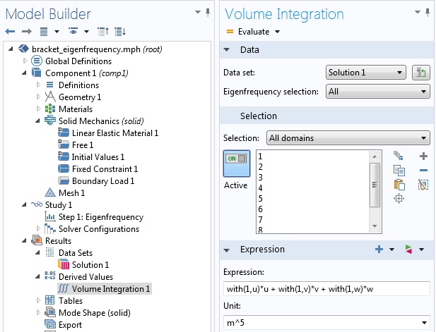
Verifying orthogonality of mode shapes using the with operator.
The above figure is from an eigenfrequency study of a 3D solid mechanics problem, where we evaluated the six lowest eigenvalues. Since we chose “All” in the Eigenfrequency selection in the Volume Integration settings window, COMSOL Multiphysics evaluates the integrand shown under “Expression” for all six values.
In each case, while the displacements u, v, and w in the x-, y-, and z-directions, respectively, are evaluated at the current eigenfrequency value that is considered, the value indexed using the with operator is evaluated at the first eigenfrequency. Thus, we expect all but the first value of this evaluation to be negligible. This is shown in the table below:
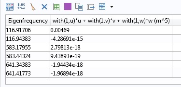
Dot product of mode shapes evaluated using the with operator.
The same idea holds true if you want to plot the difference in the solution, for example. In a solid mechanics problem, you can type with(1,v)-with(2,v) under Expression in the plot settings window to plot the difference in the y displacement of the two lowest eigenvalues. In a model with a solid mechanics problem, the COMSOL software allows you to plot a solution on a deformed configuration if you add a Deformation node to the plot. You may be wondering which values of displacement are used to obtain the deformed shape. By default, the solution corresponding to the plot’s data set is used. For eigenfrequency, frequency domain, and time-dependent studies, you can override that choice using the with operator in the Deformation settings window.
In the case of time-dependent problems, the at operator offers additional functionality during the results evaluation. Like the with operator, the at operator takes two arguments with the second argument similarly being the expression to be evaluated. The first argument is a positive real number for the actual time. For example, if 1 is used in the first argument, it means t = 1 (in the relevant unit of time) and not the lowest time the problem is solved for. If a solution has already been computed for the specified value of time, COMSOL Multiphysics uses the computed solution. Otherwise, it provides a solution at that time using interpolation.
Can the with and at operators substitute a join data set for eigenfrequency and transient analyses? The answer is that while you can reproduce certain operations on joint data sets using these two operators, solution joining has additional advantages. The with and at operators have access to solutions in the same data set only. Consider a situation where you have solved a time-dependent problem for two different initial conditions. You will have two data sets, say Solution 1 and Solution 2, each containing solutions for all time steps of the corresponding initial condition. If you want to compare the solution based on the first initial condition to the solution based on the second initial condition, you can only do this using join data sets. Moreover, solution joining gives you a new data set that you can now use as a base solution in another join operation.
In some situations, using the with or at operators can be easier than making a join data set. For instance, if you want to simultaneously work with solutions from more than two time steps from a time-dependent study, you would have to form more than one join data sets. Yet, by using the with operator you can just type, for example, with(1,u) + with(2,u) – with(3,u), where u is the quantity you are interested in, without the overhead of having to create multiple join data sets.
Concluding Remarks
In this blog entry, we have extended our discussion of solution joining for single stationary solutions to parametric, eigenfrequency, frequency domain, and time-dependent solutions. For the last three types of studies, we have also shown how the with and at operators can be used to carry out operations akin to what solution joining offers.
In particular, we have demonstrated how solution joining can be used to carry out a mesh convergence study. The norm used to evaluate convergence was the square of the difference in the dependent variable.


Comments (6)
Ivar Kjelberg
August 6, 2014Hi Temesgen
Thanks for detailed explanations, there are many useful tricks coming up in the Blog (something I have been missing since that chapter disappeared from the COMSOL journal, at least half a decade ago … 😉
Now, concerning “Joining” sequentially “time series”, is it now possible to join two time series, i.e.
Data Set 1: time 0[s] to 1[s] by step1 and another
Data Set 2: time 2[s] to 10[s] with a step 2
(or even with overlapping time values, being thus sorted out nicely ?
I believe this could be of interest for long runs, that one had interrupted for diverse reasons.
The same for egenfrequency analysis, one with the first N modes, the next with N+1 to M modes ?
Yours sincerely
Ivar
Temesgen Kindo
August 7, 2014Hi Ivar,
Thanks for the comment.
You can join solutions from two different time series. If you use a one-all combination then you can join a solution from one time step of one study with all time steps of another study. If you use all-all, you make a combination of solutions having the same indices (first time step from one with first time step from the other study and so on). This is something like “specified combinations” when you are doing multiparameter sweeps. The analog to “all combinations” which makes a Cartesian product is not available. I am guessing you expected that with an all-all joining.
Hopefully that sheds some light.
Thanks again.
Akmal Hidayat
November 5, 2014Hi Tesmegen and Ivar,
what i understand about parametric sweep is that, comsol evaluate in every single parameter or its combination as if no further evaluation has been made.
example: parameter called ‘p1’ has value 1 2 3 (no geometry, no mesh parameter) using stationary solver. The evaluation starts using p1=1. Afterwards p1=2 is evaluated and comsol could not ‘remember’ that some of the results are already caculated for p1=1. Or the result from p1=1 may only need to be ‘adapted’ to have result of p1=2.
i’m sure that comsol uses same equation, so that compiling equation is not necessary; and same dependent variables.
or i misunderstood about what comsol does with parametric sweep.
best regards
akmal
Temesgen Kindo
November 5, 2014Dear Akmal,
Thank you for your comment.
When you do a regular parametric sweep, COMSOL solves the problem for each parameter from scratch. However, if you need to use the solution from a previous parameter value as a trial solution for the current parameter in a nonlinear problem then you should use an Auxiliary Sweep.
If you click on a study step, you will see on its settings window a section “Study Extensions”. If you expand that section, you will find “Auxiliary sweep”. That is what you use if you are, for example, load ramping and want to use the solution from the previous load step as a trial solution in the current nonlinear iteration.
Hopefully that clears things up. Let us know if you have further questions.
Mateusz Celmer
September 3, 2016Dear Akmal,
thank you for interesting and detailed article!
My question is about looping an animation over both time and a result parameter. I am wondering if it is possible to make an animation with changing Camera View (rotating, zooming, moving) in the Time Dependant simulation. I found a method for adjusting the camera view using a “result parameter” but you have to choose to loop the animation either over time or the parameter (never both). After you choose the result parameter, the time depenant simulation is freezed.
I have been looking for the answer for a long time. After I found this article I thought that you may know the answer.
Yours sincerely,
Mateusz
Mateusz Celmer
September 3, 2016“Dear Temesgen” of course 🙂