
You can use topology optimization to get ideas for the device geometry early on in the design phase, for example, when designing a Tesla microvalve. The setup of this optimization problem was simplified with the introduction of the Density Model feature as of COMSOL® version 5.4. In this blog post, we show how to use the shape optimization features available as of COMSOL® version 5.5 to improve on a simple design inspired by the more complex topology optimization result.
Theory Behind Tesla Valves
Tesla valves are devices with large anisotropic flow resistance; i.e., it is significantly easier to push the fluid through in one direction compared to the other direction. Therefore, the devices can be used as leaky valves that are very robust, owing to the lack of moving parts.
You can consider having the same pressure drop for the two flow directions and optimizing the flow rate ratio, but depending on the context, it might be more relevant to fix the flow rate ratio and optimize the pressure drop ratio. This is exemplified in the Optimization of a Tesla Microvalve tutorial model.
Thus, the number that is maximized is the diodicity, Di, defined as
where \Delta p_{\leftarrow} and \Delta p_{\rightarrow} are the pressure drops in the two flow directions.
The performance of Tesla valves exploits the nonlinear nature of inertial effects, so if the flow rate is small, inertial effects will vanish, causing the physics to become linear. In such a flow regime, the valve will not work —— the diodicity will be 1. The strength of the nonlinearity can be quantified with the Reynolds number, Re, defined as
where \rho is the density, \mu is the viscosity, U_\mathrm{in} is the characteristic velocity, and D is the characteristic length scale.
Reynolds numbers above 1000 tend to cause transient flow patterns, while inertial effects are too small for Reynolds numbers below 10. Therefore, to have a stationary flow with significant inertial effects, a Reynolds number of 100 is chosen for the optimizations. However, this does not mean that the device performance will deteriorate if the flow rate is increased.
Performing a Topology Optimization in COMSOL Multiphysics®
Topology optimization can divide a domain into solid and fluid regions. When using the density method, this is achieved by interpolating material parameters. This means that the solid regions are approximated as sponges with a very low permeability. Thus, the design variable, 0\leq\theta_c\leq1, controls a damping force, \mathbf{F}_\mathrm{Darcy}, defined as
where \alpha(\theta_c)is large for \theta_c=0 and zero for \theta_c=1, corresponding to solid and fluid regions, respectively.
Due to the Helmholtz filtering, the damping can become small, but only zero if everywhere.
In practice, the damping term should not vary completely arbitrarily, because this can give rise to unphysical numerical effects. To limit the variation of the damping term, we introduce a minimum length scale using a Helmholtz filter. (See a previous blog post on the density method for more information.)
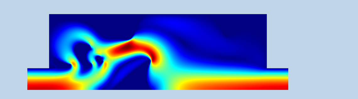
The result of the topology optimization is shown in the figure below. You can see that the damping term is not sufficiently high near the corners of the central triangle because the No Slip boundary condition is violated. You can perform a verification study to investigate how much the performance depends on this unphysical effect, either by increasing the damping or creating a new component without the solid regions. In this case, the finite permeability seems to have a minor effect on the performance.
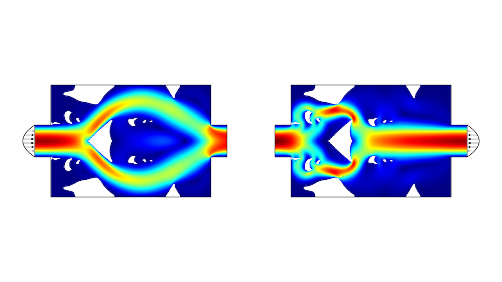
Figure 1. The topology optimization results are shown in colors with solid regions in white and the fluid region colored according to the flow velocity. The flow pattern is significantly simpler for the easy flow direction, resulting in a pressure drop ratio of 2.4.
Performing a Shape Optimization of a Tesla Microvalve
The results of the topology optimization can sometimes be very complex, and it might be possible to make a much simpler design with similar performance, as shown below. The design features the same basic principle with a central obstacle near a contraction of the channel. There is also a free line to divert the flow on a longer path, when it is coming from the right.
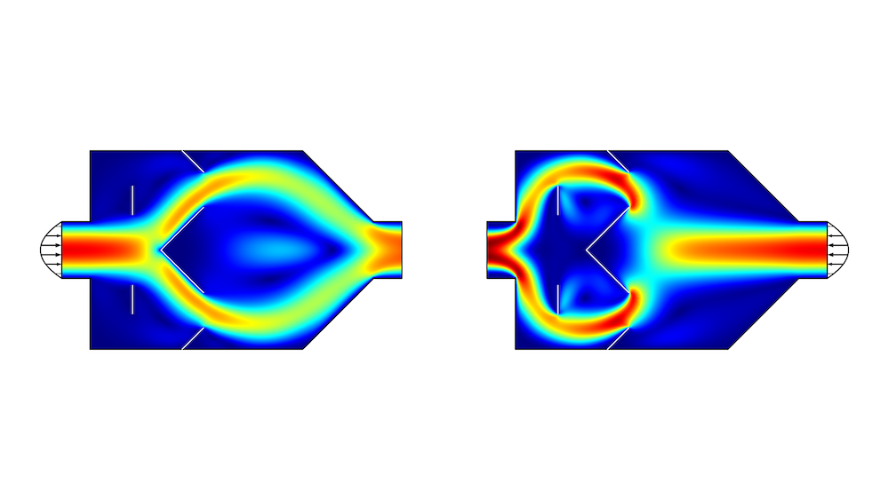
Figure 2. The flow velocity is plotted in a simple geometry that uses interior walls (white lines). The pressure drop ratio is equal to 2.3.
The COMSOL Multiphysics® software supports gradient-based shape optimization by fixing the mesh topology; i.e., only the position of the mesh nodes changes. The Optimization Module, as of COMSOL Multiphysics version 5.5, comes with several built-in features for shape optimization. The Polynomial Boundary feature is one of them. It handles the deformation of interior nodes by a smoothing equation, while the deformation of the interior walls is given by
where d_\mathrm{max} is the maximum displacement, B_i^n is the i‘th Bernstein polynomial of n‘th order, while 0\leq s \leq 1 is the COMSOL s parameter.
Bernstein polynomials satisfy the bounds of their coefficients across the whole line, which means that each point on the line is confined to move in a square box with side length 2d_\mathrm{max}.
If the displacement is small and first-order polynomials are used, the lines will stay straight and move little, leading to a marginal improvement of the objective function. If, on the other hand, the maximum displacement is large and a high polynomial order is used, issues with the mesh quality are guaranteed to arise, so you have to find a balance. The figure below shows the result of shape optimization with second-order polynomials and a maximum displacement equal to the initial length of the left interior wall.
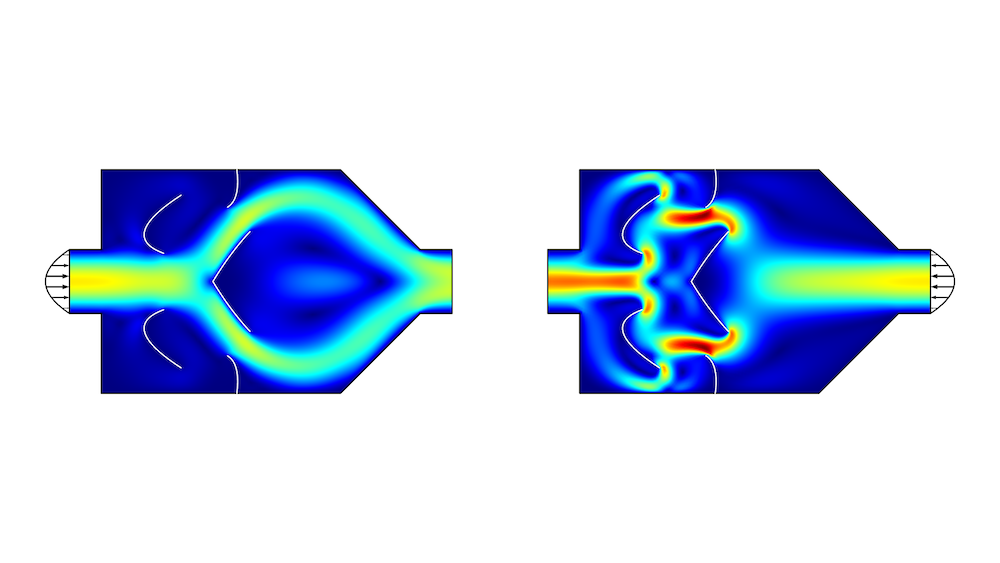
Figure 3. The flow velocity is plotted in the shape-optimized geometry. The pressure drop ratio is equal to 3.5.
The shape-optimized design is significantly simpler than the result of the topology optimization (Figure 1), but the performance is significantly worse. The Tesla microvalve is an example where it is possible to improve on the result of the topology optimization by applying shape optimization as a postprocessing step.
Rather than using interior walls with gradient-based optimization, you might make obstacles consisting of solid objects and apply a derivative-free optimization. This is shown in the Parameter Optimization of a Tesla Microvalve tutorial model.
This model, as well as the ones shown here, exploits symmetry, but the original Tesla valve by Nicola Tesla was not symmetric (Ref. 1), so it is natural to ask if the performance can be improved by removing the symmetry constraint. You might also ask if having a pressure-driven flow and optimizing the flow rate ratio will lead to a different design, or how much the shape-optimized design could be improved by introducing more interior walls. It is easy to ask the questions, and with COMSOL Multiphysics, we can also find the answers.
Next Steps
Learn more about how the capabilities of the Optimization Module can fit your design needs.
Reference
Valvular Conduit, Nicola Tesla, 1920, US Patent 1,329,559.

Comments (1)
Levente Szalontai
November 18, 2019Are WE saying that we will be capable to build small computers powered by WATER? 😉