

In 1961, R. Fitzhugh (Ref. 1) and J. Nagumo proposed a model for emulating the current signal observed in a living organism’s excitable cells. This became known as the FitzHugh-Nagumo (FN) model of mathematical neuroscience and is a simpler version of the Hodgkin-Huxley (HH) model (Ref. 2), which demonstrates the spiking currents in neurons. In today’s blog post, we’ll examine the dynamics of the FN model by building an interactive app in the COMSOL Multiphysics® software.
A Nerve Cell’s Action Potential
Nerve cells are separated from the extracellular region by a lipid bilayer membrane. When the cells aren’t conducting a signal, there is a potential difference of about -70 mV across the membrane. This difference is known as the cell’s resting potential. Mineral ions, such as sodium and potassium, and negatively charged protein ions, contained within the cell, maintain the resting potential. When the cell receives an external stimulus, its potential spikes toward a positive value, a process known as depolarization, before falling off again to the resting potential, called repolarization.
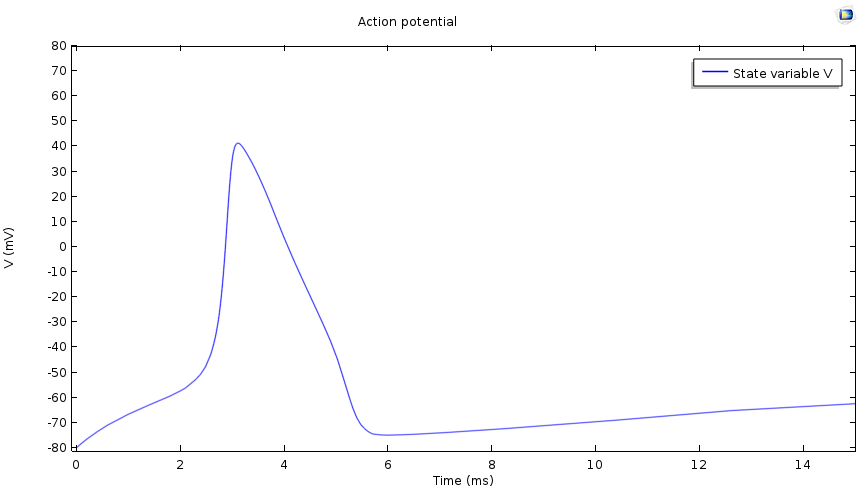
Plot of a cell’s action potential.
In one example, the concentration of the sodium ions at rest is much higher in the extracellular region than it is within the cell. The membrane contains gated channels that selectively allow the passage of ions though them. When the cell is stimulated, the sodium channels open up and there is a rush of sodium ions into the cell. This sodium “current” raises the potential of the cell, resulting in depolarization. However, since the channel gates are voltage driven, the sodium gates close after a while. The potassium channels then open up and an outbound potassium current flows, leading to the repolarization of the cell.
Hodgkin and Huxley explained this mechanism of generating action potential through mathematical equations (Ref. 2). While this was a great success in the mathematical modeling of biological phenomena, the full Hodgkin-Huxley model is quite complicated. On the other hand, the FitzHugh-Nagumo model is relatively simple, consisting of fewer parameters and only two equations. One is for the quantity V, which mimics the action potential, and the other is for the variable W, which modulates V.
Today, we’ll focus on the FN model, while the HH model will be a topic of discussion for a later time.
Defining the FitzHugh-Nagumo Model
The two equations in the FN model are
and
The parameter I corresponds to an excitation while a and b are the controlling parameters of the model. The evolution of W is slower than that of the evolution of V due to the parameter ε multiplying everything on the right-hand side of the second equation. The fixed points of the FN model equations are the solutions of the following equation system,
and
The V-nullcline and W-nullcline are the curves V-V^3/3-W + I and V+a-bW, respectively, in the VW-plane. Note that the V-nullcline is a cubic curve in the VW-plane and the W-nullcline is a straight line. The slope of the line V+a-bW is controlled in such a way that the nullclines intersect at a single point, making it the system’s only fixed point.
The parameter I simply shifts V-nullcline up or down. Thus, changing I modulates the position of the fixed point so that different values of I cause the fixed point to be on the left, middle, or right part of the curve V-V^3/3-W + I.
Understanding the Dynamics of the FN Model
To simulate what happens when the fixed point is in each region, we can use the Global DAE interface included in the base package of COMSOL Multiphysics®.
The V-nullcline is shown in the figure below in a green color. In the region above this nullcline \frac{dV}{dt}<0, while in the region below it is positive. The W-nullcline is shown in red; in the region to the right of this straight line, \frac{dW}{dt}>0, and to the left, \frac{dW}{dt}<0.
Let’s first examine what happens if the fixed point is on the right side, Region 3, of the V-nullcline. We’ll say that when t, representing time, equals zero, both V and W are also at zero. In this case, both \frac{dV}{dt} and \frac{dW}{dt} are positive at and around the starting point and thus both change as time progresses. But since V evolves faster than W, V increases rapidly while W remains virtually unchanged. In the figure, we can see that this results in a near-horizontal part of the V-W curve.
As the curve approaches the V-nullcline, the rate of change of V slows down and W becomes more prominent. Since \frac{dW}{dt} is still positive, W must increase, and the curve moves upwards. The fixed point then attracts this curve and the evolution ends at the fixed point.
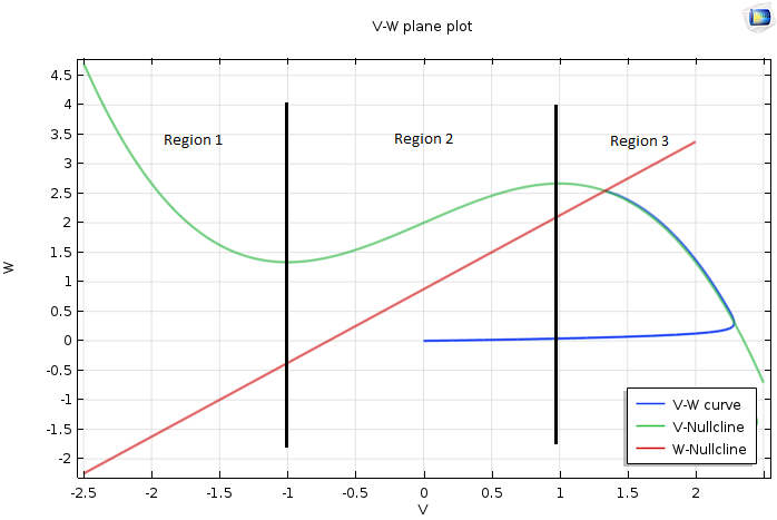
Plot of the VW-plane when the fixed point is on the right side of the V-nullcline.
If the fixed point is in the middle, Region 2, then what we have discussed so far holds true. The difference is that once the curve goes beyond the right knee of the V-nullcline, \frac{dV}{dt} becomes negative and V rapidly decays. While moving left, the curve crosses the red nullcline from right to left. From this point on, while both V and W diminish, the evolution of V dominates and the curve becomes horizontal once again.
This continues until the curve hits the left part of the V-nullcline. The curve begins to hug the V-nullcline and starts a slow downward journey. When it touches the left knee of the V-nullcline, it moves rapidly toward the right part of the V-nullcline. Note that this motion never hits the fixed point and therefore keeps repeating, which we can see in the plot below.
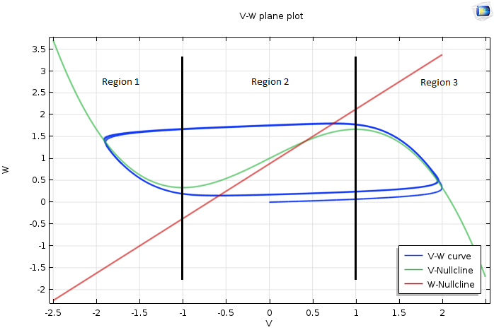
Plot of the VW-plane when the fixed point is in the middle region of the V-nullcline.
That leaves us with one last case to discuss — when the fixed point is on the left part, Region 1, of the V-nullcline. The results should look like the following plot. Note that the analyses we previously performed carry over.
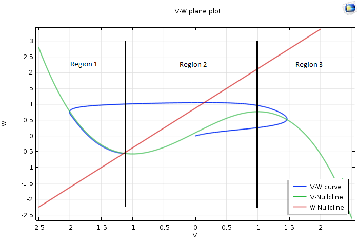
Plot of the VW-plane when the fixed point is on the left side of the V-nullcline.
Simulating the FN Model Using the Application Builder
To explore the rich dynamics of the FN model described above, we need to repeatedly change various inputs without changing the underlying model. As such, a user interface that allows us to easily change the model parameters, perform the simulation, and analyze the new results without having to navigate the Model Builder tree structure to perform these various actions is desirable.
To accomplish this, we can turn to the Application Builder. This platform allows us to create an easy-to-use simulation app that exposes all of the essential aspects of the model, while keeping the rest behind the scenes. With this app, we can rapidly change the parameters via a user-friendly interface and study the results using both static figures and animations. The app also makes it easy for students to understand the FN model’s dynamics without having to worry about creating a model.
The important parameters of the FN model, i.e. a, b, ε, and I, are displayed in the app’s Model Parameters section. The graphical panels display various quantities of interest such as the waveform for V and W. We display the phase plane diagram in the top-right panel along with the V– and W-nullclines. The position of the fixed point is easily identifiable from that plot. Once the simulation is complete, we can animate the time trajectories by choosing the animation option from the ribbon toolbar. To get a summary of the simulation parameters and results, we can select the Simulation Report button.

App showing the dynamics of the FitzHugh-Nagumo model when the fixed point is in Region 2.
We can easily reproduce the cases described in the previous section with our app. The image above, for example, shows what happens when the fixed point is in Region 2. We can easily move the fixed point to either Region 1 or 3 by making the current 0.1 or 2.5, respectively. Note that any other parameters in the app can also be changed to see if other interesting trends emerge.
The app that we’ve presented here is just one example of what you can create with the Application Builder. The design of your app, from its layout to the parameters that are included, is all up to you. The flexibility of the Application Builder enables you to add as much complexity as needed, in part thanks to the Method Editor for Java® methods. In a follow-up blog post, we’ll create an app to illustrate the dynamics of the more complicated HH model. Stay tuned!
References
- FitzHugh R. Impulses and Physiological States in Theoretical Models of Nerve Membrane. Biophysical Journal. 1961;1(6):445-466.
- Hodgkin AL, Huxley AF. A quantitative description of membrane current and its application to conduction and excitation in nerve. The Journal of Physiology. 1952;117(4):500-544.
Further Resources on Using the Application Builder
- See how to combine equation-based modeling and apps in this blog post: Implementing the Weak Form with a COMSOL® App
- To find out how to build your own app, check out our Intro to Application Builder Videos series
Oracle and Java are registered trademarks of Oracle and/or its affiliates.

Comments (2)
atul tanaji Mohite
December 13, 2019Can you please share the COMSOL file you have used to simulate and create these plots?
Regards
Emily Ediger
December 17, 2019Hi there! These files are no longer available. If you have any questions, please reach out to support by email at support@comsol.com or online at https://www.comsol.com/support.