

Dimples are famously crucial for the aerodynamic properties of a golf ball: They generate a turbulent flow that reduces the ball’s drag. However, doesn’t this sound counterintuitive? In general, smooth objects are more aerodynamic than rough ones. In today’s blog post, we will dig into the details of this apparent paradox; learn how to use this knowledge to model the trajectory of a golf ball with the COMSOL Multiphysics® software; and, finally, find the best angle to hit the ball. Keep reading for a hole in one…
From Observation to Mathematical Model
As a child, I occasionally would walk around a nearby golf course with my family on rainy days; the only times when no golfers would dare to play. Our own game was to find lost balls from previous, unfortunate players. The person who found the most balls would win. After many rainy days, our collection of golf balls grew bigger and bigger! Although none of us knew how to play golf, we assumed that the dimpled shape of the ball was there for a reason, probably for aesthetics or to make the ball fly faster through the air.
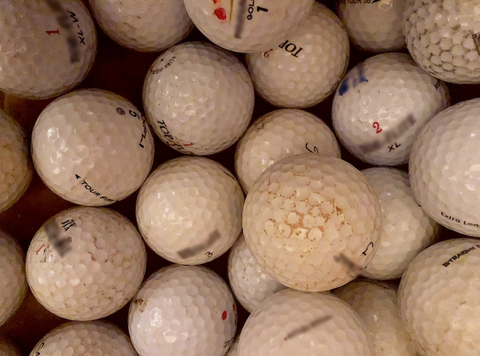
Ever wonder why golf balls have dimples?
Years passed, and now I am the unfortunate golfer losing golf balls on the golf course (I guess life has come full circle). However, I now have the possibility to take a second look at those familiar spheres through the prism of an engineer’s eyes: Why do they have dimples? Can I model a golf ball with COMSOL Multiphysics? Can I optimize my shot in order to lose fewer balls — and possibly make a par? A previous blog post already helped me improve my golf swing, but I needed more information, so I went back to my textbooks…
The Drag Crisis Observation
Throughout history, the flows around many different shapes have been studied by scientists. For example, vortex streets are generated by the flow around cylinders. Although a sphere does not generate this type of large alternating flow structure, the flow characteristics can also be linked to the Reynolds number. For a sphere of diameter d in a fluid of density \rho, dynamic viscosity \mu, and velocity U, it is defined as:
(1)
For low values of the Reynolds number, the flow is said to be laminar and the viscous forces are dominant. On the other hand, if the Reynolds number is large, the flow is turbulent and the inertial forces are dominant. Instead of comparing absolute values of the drag D, i.e., the resistance of an object against the flow, it is a common practice to define a nondimensional drag coefficient C_D as:
(2)
Where A= \dfrac{1}{4} \pi d^2 is the cross-sectional area of the ball.
It was observed almost simultaneously by Gustave Eiffel and Ludwig Prandtl that, depending on the flow regime, the coefficient for a sphere is not constant and even dramatically different within a short range of Reynolds numbers. This sudden drop in the drag coefficient is often called drag crisis and is observed for other type of balls, like football and soccer balls. The only difference is its location, as can be seen in the following image.
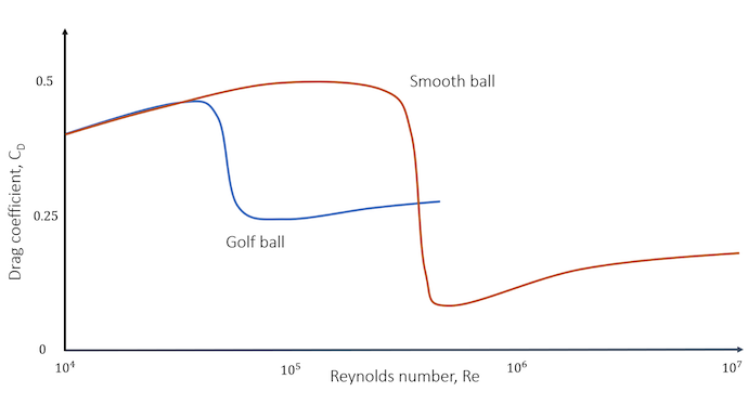
Comparison of the drag coefficient distribution between a smooth ball and a golf ball. The dimples have shifted the drag crisis toward lower values of Reynolds, but the drop is less important compared to a smooth ball. Note also that the golf ball’s drag coefficient is only smaller for a limited range of Reynolds values.
Knowing that a typical speed for a golf ball hit by a driver is around 260 km/h (160 mph), and considering an official golf ball design (d= 42.67 mm), this gives a typical Reynolds number of 2\cdot10^5. As can be deduced from the previous graph, this makes the drag coefficient fall in the perfect range of the Reynolds number: around half the value of a smooth ball. This explains the reason for the dimples on golf balls. For the specific range of Reynolds numbers the golf ball will experience, the drag is lower — therefore, the ball can go further.
You might not be satisfied with this answer. We have observed that golf balls with dimples have lower drag, but we have not yet explained the reason why the drag crisis happens at lower speeds. To understand this phenomenon, we must take a closer look at the flow around the sphere.
The Reason for the Drag Crisis
First of all, let’s recall that the drag of an object is caused by two sources:
- Pressure drag, also referred to as form drag, generated by the distribution of pressure around the body
- Viscous drag generated by shear stresses along the boundaries
For blunt bodies, such as a smooth ball, the pressure drag is most significant at the range of studied Reynolds numbers. Consequently, the pressure distribution around the sphere will determine its total drag.
Without going too much into the theory of turbulence, a laminar boundary layer is first developed at the front of the sphere (the flow is separated in different layers that almost do not exchange mass or momentum). From this point, there are two options, depending on the type of flow:
- If the flow is laminar enough (low Reynolds number), the boundary layer will not have time to transition to a turbulent boundary layer before it separates due to an adverse pressure gradient at an angle approximatively equal to 82 degrees, creating a large wake behind the sphere.
- If the flow is turbulent enough, the boundary will have time to transition to turbulence before the critical 82 degrees. When this happens, the flow is better mixed, which enables an exchange of momentum from the top part of the boundary layer. This has the effect of energizing the bottom part of the boundary layer, increasing the velocity gradient near the wall, and delaying the flow separation to an angle of around 120 degrees. It looks like the flow “sticks” better to the surface.
Comparison of the turbulent wake behind a golf ball and a smooth sphere. The Reynolds number is around 1e5.
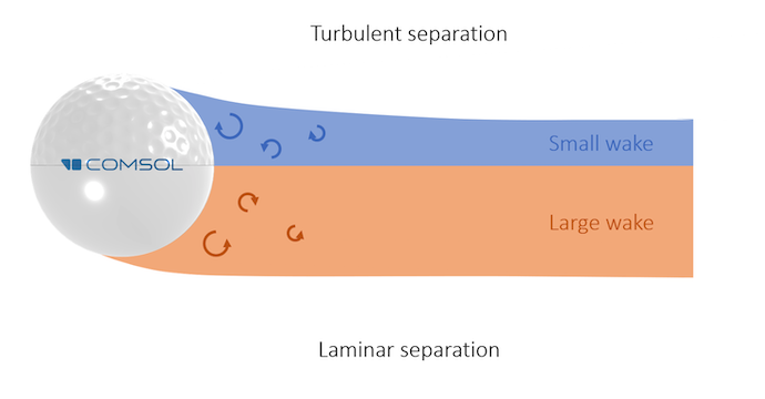
Comparison of the turbulent wake behind a dimpled golf ball (top), which originates from a turbulent boundary layer separation, and a smooth ball (bottom), which originates from a laminar boundary layer separation. Note that the separation point for the dimpled ball is located much further downstream and the wake is smaller.
A lot of energy is lost in a turbulent wake, making the pressure drop significantly. Hence, the pressure drag of a sphere, which is the dominant drag, is mainly affected by the size of the wake region. From this information, the drag coefficient graph should now make much more sense. For the golf ball:
- The transition from the laminar to turbulent boundary layer occurs for lower Reynolds numbers, due to small vortices induced by the dimples. This generates a smaller wake and therefore a smaller drag.
- The drag crisis is not as deep compared to a smooth ball. For a similar wake size, the rough surface makes the viscous drag from the front part less negligible.
Modeling the Aerodynamic Forces of Golf Balls
Now we understand why golf balls have dimples in the first place. Let’s remember that the drag is lower and therefore the ball can go further. To find out how much further the ball can go, we first need to compute its trajectory. The forces acting on the ball and the initial conditions are depicted in the following figure, neglecting the effect of buoyancy, since the ball is almost 1000 times heavier than the corresponding volume of air.

Initial condition and forces acting on a golf ball shot.
The initial condition can be taken from the end results of a previous performance analysis, where the ball is hit by a 7-iron with a shaft speed of 145 km/h (90 mph):
- Initial ball speed: 187 km/h (116 mph)
- Initial spin rate: 6113 rpm
- Initial launch angle: 17.4°
Using Newton’s second law on the ball of mass m, noting \overrightarrow{a} its acceleration and \overrightarrow{F_g} the gravity force:
(3)
The norm of the drag D is computed by rearranging Eq. 2:
(4)
Similarly, the lift L produced by the Magnus effect is defined by a lift coefficient C_L that depends on the spin rate \omega of the ball:
(5)
The dependency of the lift coefficient in the spin rate of the golf ball has been extensively studied by Bearman and Harvey in 1976 (Ref. 1). They also observed that the drag coefficient should also depend on the rotation (the curve from the first figure is valid for one specific spin rate). For a more general description, a nondimensional spin factor S, the ratio between the peripheral speed and the flow speed, is introduced:
(6)
While it could be argued that the results were obtained for older golf balls and the curves might be different nowadays, the results from Bearman and Harvey are covering the largest range of Reynolds numbers and spin factors in available literature. Consequently, the results that are obtained in this blog post should not be taken as true values for modern golf balls. The following curves were obtained by fitting a cubic polynomial curve with the Using COMSOL Models Together with Curve Fitting app on the data taken from Figure 9 of Ref. 1 using the Curve Digitizer app:
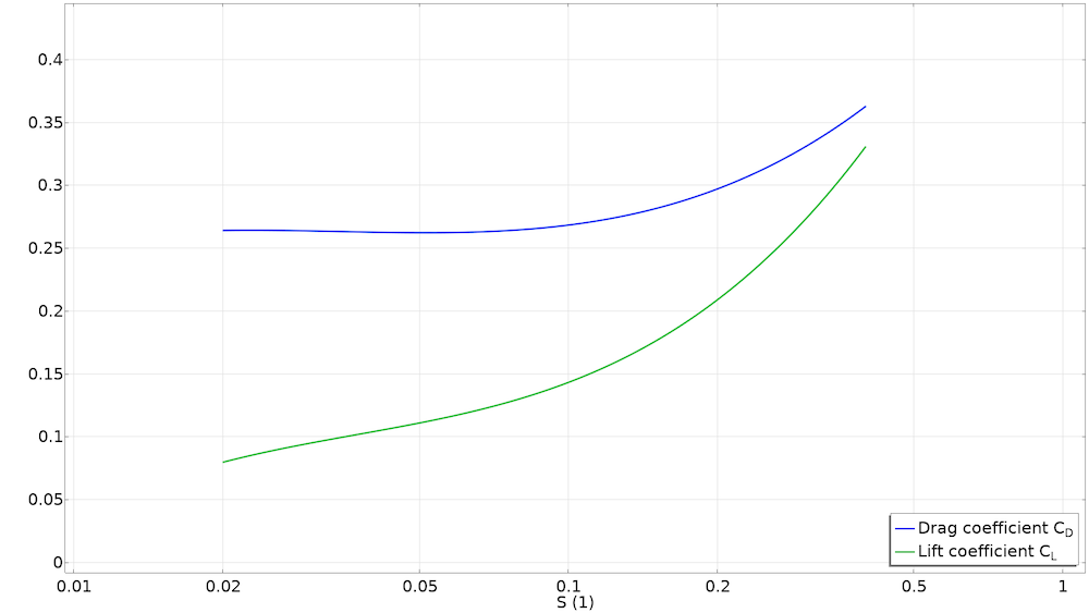
Drag and lift coefficient distribution in terms of the spin factor.
The drag coefficient for the smooth ball is taken from the Standard drag correlations (see the first image) and the lift coefficient is approximated as being equal to that of the spinning golf ball (in reality this coefficient is smaller).
Finally, since the rotation will be slowed down due to friction, the spin rate can be modeled using an exponential decay, as proposed by Smits and Smith (Ref. 2).
(7)
where c=10^{-4} is an experimental constant.
Considering that the drag is opposite to the motion of the ball and the lift perpendicular, we arrive at the following set of equations by projecting on the x– and y-axes:
(8)
\ddot{x} = -\dfrac{\rho AU}{2m} \left( C_D \dot{x} + C_L \dot{y}\right)\\
\\
\ddot{y} = \dfrac{\rho AU}{2m} \left( C_L \dot{x} – C_D \dot{y} \right) -g
\end{array}\right.
with U=\sqrt{\dot{x}^2+\dot{y}^2}.
This system of equations consists in a set of ordinary differential equations (ODE), which might look complicated due to the dependencies between all of the variables. However, it is actually straightforward to implement and solve with COMSOL Multiphysics.
Implementing the Golf Ball Model in COMSOL Multiphysics®
The easiest way to implement this problem is by using the Events interface in a 0D component that can both solve the system of Eq. 8 using a Global Equations node and also stop the computations when the ball touches the ground (y=0).

Setting up the variables used by the study.
The first step is to set up the different variables that are used by the study. Here, they are computed through different functions and global parameters. In particular, the parameter smooth determines the type of ball being launched:
- Dimpled golf ball (
smooth=0) - Smooth ball (
smooth=1)
The quantities xt and yt are the time derivatives of the position, computed by the Events interface.

System of global equations solving for the position of the ball.
The second step is to set up the system of Eq. 8 using the corresponding initial conditions. Since all of the parameters and variables are already defined, this step is straightforward.
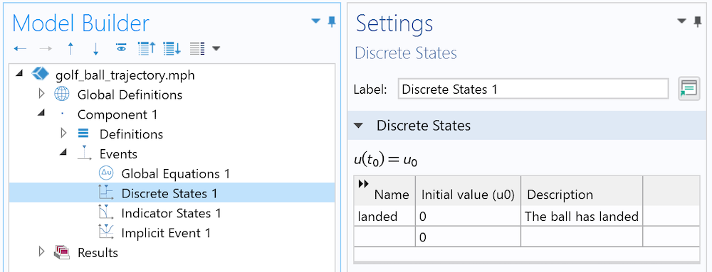
The Discrete State interface is used to define whether the ball has landed or not.
Like in a previous blog post, a Discrete State variable, which is best suited for on/off conditions, is added. This represents the global state of the ball: Either it has landed or not. Initially, the ball is considered as not landed, so landed=0.
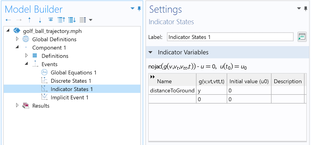
The Indicator States interface is simply the current height. The Discrete State is turned on once the ball has landed.
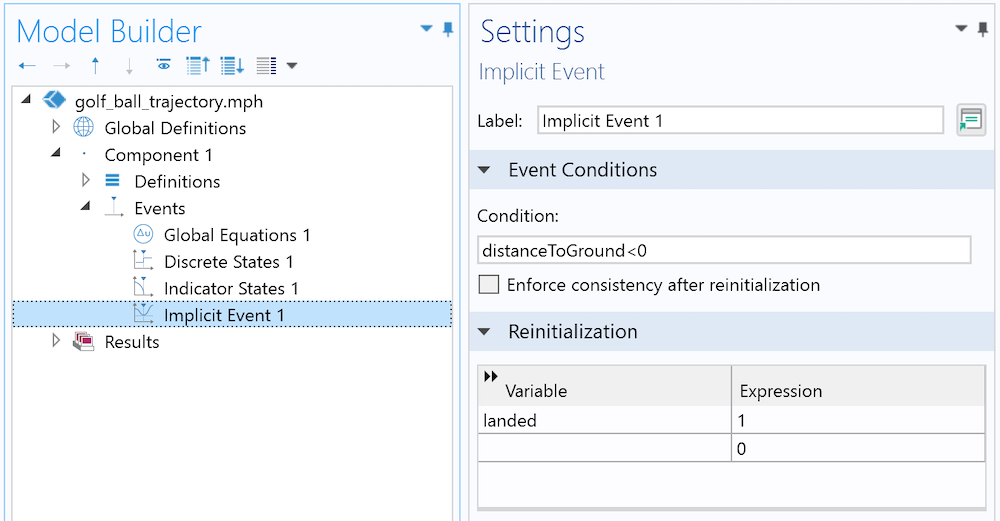
The Discrete State has to be updated only when the ball touches the ground. We don’t know in advance when this event will happen, but we can translate it mathematically (the height becomes negative). This is the exact purpose of an Implicit Event node: When an Indicator State (here, the current height) satisfies a certain condition, the event is triggered.

The solver sequence is modified in order to add the Stop condition.
The final step is to create a Study node. A Parametric Study can be used to sequentially compute the golf ball and the smooth ball, and a time-dependent study can be used to solve for the trajectory of the ball. The solver sequence from the time-dependent study needs to be modified in order to stop the computations when the event has been activated.
Simulation Results
Now that everything is set, let’s run the study!
Real-time animation of the trajectory of a golf ball and a smooth ball hit by a 7-iron. The dimpled ball experiences a much lower drag (the color legend shows the drag coefficient) compared to the smooth ball. Note that the ball experiences the drag crisis at the top of the trajectory, where the velocity (hence the Reynolds number) gets lower.
Notice that the shape of the trajectory is not a parabola, as one could have found if the drag or lift had been neglected. The ball first rises almost in a straight line before dropping abruptly after reaching the maximum height. It is possible to see from the results that the ball with dimples goes 25% further (30 meters or 33 yards) compared to the smooth ball. In other words, the green is now much closer and no additional force was needed!
The explanation comes from the fact that the drag force, acting against the motion of the ball, is much smaller for the golf ball (for a reason addressed at the beginning) throughout the flight. When the ball reaches its maximum height, the potential energy, which is proportional to the height, is also at its maximum. This energy transfer is done in detriment of kinetic energy; the ball goes slower. Hence, the Reynolds number decreases (or equivalently, the spin factor increases) and the drag increases as a consequence.
Regarding the absolute carry distance of around 150 m (165 yds), this is much larger than the typical golf shot of an average player (128 m or 140 yds) but in the lower bounds of a typical shot of a PGA player. This result is reasonable, considering that the drag and lift data does not originate from modern golf balls.
Finding the Optimal Launch Angle
The effect of the dimples on a golf ball should now be clear: They make the ball go further. However, in practical terms, this does not say much about how I should hit the ball. What is the launch angle that I should impose on the ball, with the hypothesis that the shaft speed and angle of attack are constant, so that the carry distance is optimized? A first approach would be to run a parametric study, or even an optimization study, to find this value. Here is a graph that shows the carry distance depending on the launch angle for a given angle of attack and spin rate.
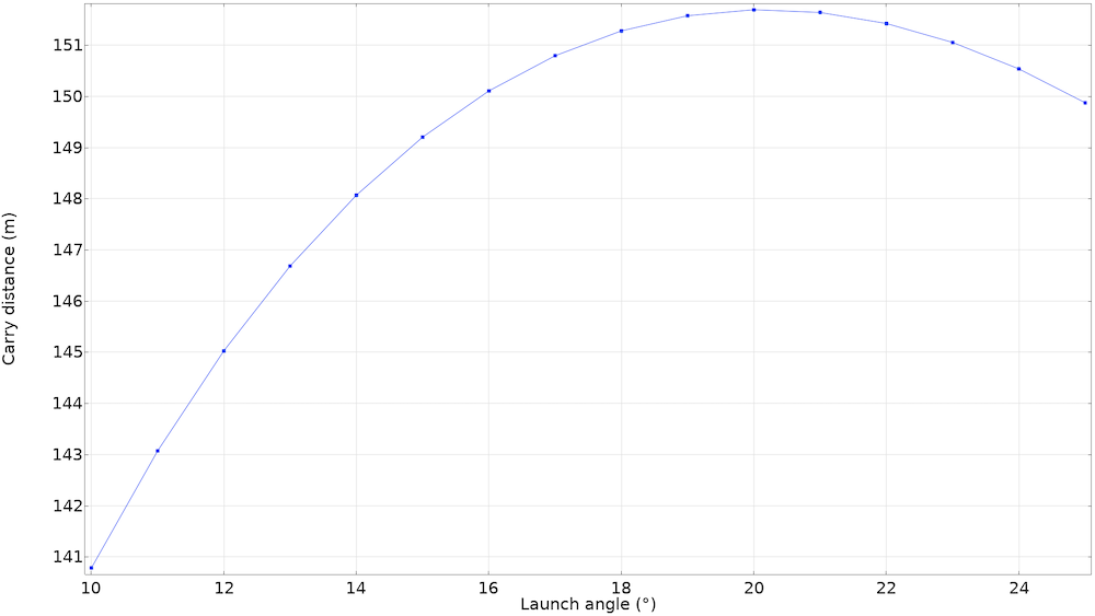
Results from the parametric study, using an angle of attack of -4.3° and an initial spin of 6113 rpm with a 7-iron. It looks like the best launch angle should be around 20°.
From this figure, it would seem that the best angle of attack is around 20°. However, PGA golfers (who, in theory, should on average approach the optimized angle) are shooting on average at an angle of 16°. What is going on here? Our hypothesis of a constant spin rate is wrong: Hitting the ball at a larger launch angle means that the club face needs to be “more horizontal” when hitting the ball. Just like when the ball is “sliced” in tennis, the golf ball spins faster due to higher friction, but goes slower.

Comparison between two dynamical lofts for a constant angle of attack. The angles are measured compared to a horizontal line. The launch angle increases when the dynamical loft increases. Since the angle between the dynamical loft and the angle of attack (often called “spin loft”) gets larger, the ball will spin faster.
Finding the relationship between the launch angle, spin rate, and ball velocity is not direct and does not necessitate results from either experiments or simulation. Here, since we have a golf ball model ready, let’s use it by parameterizing it!
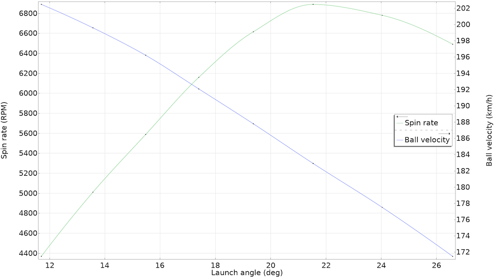
Results from the parameterized version of the tutorial model. The points are interpolated using a cubic spline for a smoother curve. As expected, the spin rate increases for larger launch angles and the velocity has the inverse behavior.
The results have to be taken with precaution. A more detailed study should be carried out to include a mesh convergence study, comparison with the curves of other shafts, etc. Nonetheless, the results conform to reality enough.
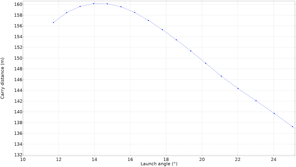
Carry distance for a 7-iron, depending on the launch angle for an angle of attack of -4.3° with nonconstant spin. The curve has been shifted to lower values of the launch angle to better capture the real-world behavior.
The parametric study can now be run again with the correct values of spin and velocity. Note that the curve has been shifted to the left. In other words, it seems that decreasing the launch angle (hence the dynamical loft) helps by reducing the spin and giving the ball a higher translational kinetic energy. The curve is not centered around 16°, as one would expect. However, to obtain this result, many hypotheses have been made (such as the distribution of drag and lift and the spin rate dependency) that greatly influence the end results. More data about modern golf balls and ball impact analyses would help to obtain more accurate results.
Conclusion
In today’s blog post, we answered a seemingly simple question about golf ball dimples, which has to do with the behavior of the turbulent boundary layer over a sphere at a specific range of Reynolds numbers. This also outlines a classical process in engineering. The observation of a common object led us to a deeper understanding of a complex physical phenomenon, which in turn led us to model and verify it under some assumptions with COMSOL Multiphysics. Finally, we found an optimal launch angle and extracted useful information for the real world.
For our golfer audience, who have probably asked similar questions to mine, the lesson to remember is to try to lower your dynamical loft while keeping the same angle of attack, in order to decrease the spin rate. While the simulation results make it sound simple, I am not sure how exactly to do this on the fairway. Therefore, the real lesson of this blog post is to ask a professional golf teacher, not a simulation engineer!
Try It Yourself
Try computing the trajectory of a golf ball in COMSOL Multiphysics. Click the button below to access the model file featured in this blog post:
References
- P. Bearman and J.K. Harvey, “Golf ball aerodynamics”, Aeronautical Quarterly, vol. 27, no., pp. 112–122, 1976.
- A.J. Smits and D.R. Smith, “A new aerodynamic model of a golf ball in flight”, Science and Golf II, Taylor & Francis, pp. 433–442, 2002.

Comments (3)
Mathias REMY
October 6, 2021Hello,
Thanks for this very interesting article.
Just a remark: I think there is a mistake on equation 5 (lift coefficient L). It is identical to equation 4 whereas it shouldn’t be.
Best Regards
Bixente Artola
October 6, 2021 COMSOL EmployeeHello Mathias, thank you for your comment!
The lift and drag have indeed -almost- the same expression, as they are both expressed in terms of the dynamic pressure (q=1/2*rho*U^2) and the reference area. The major difference being the coefficients CD and CL, which are scaling the expressions (you can find their distribution in terms of the Reynolds number or the spin factor in this blog post). This allow to incorporate all the complex 3D phenomena into one simple expression.
Bixente
Mathias REMY
October 6, 2021Hello Bixente,
My bad! Sorry about that, I guess I read it a bit too quickly.
Thanks for your quick feedback. All clear now.
Mathias