

Suppose you have some CAD description of a part that will be deformed, such as a flexible printed circuit board. These CAD parts are designed in their undeformed, as-manufactured state. However, for analysis purposes, we are only interested in the deformed, as-assembled state. Here, we will look at a set of techniques for wrapping and warping such geometries as well as modeling the space around the deformed part. Let’s learn more!
Defining a Deformed Shape
Let us consider the example geometry shown below: a thin rectangular strip of flexible material with a pattern of electrodes on one side. This is similar to what we might see in a capacitive sensor. For more complicated patterns, you could use the DXF import capabilities of the core package of the COMSOL Multiphysics® software, or the ECAD import capabilities of the ECAD Import Module.
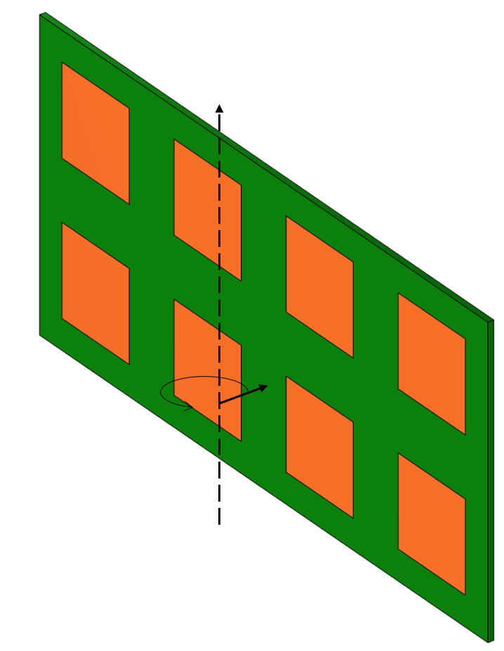
A flexible part that will be wrapped around one axis.
We will define a deformation of this part under the assumption that this imposed deformation is sufficiently similar to the actual deformation that we would get by solving for the geometric nonlinear (and possibly material nonlinear) solid mechanics governing equations. That is, we will avoid having to solve for the deformations by assuming a deformation field.
We will consider singly curved deformations, so we can frame the discussion by looking at a 2D plane, normal to the bend axis, as shown in the image below. What we would like is to deform this thin part such that its centerline length, and hence the volume, do not change. This is easily done by defining a mapping between the undeformed state of the part, in Cartesian coordinates, and the deformed state, in cylindrical coordinates.
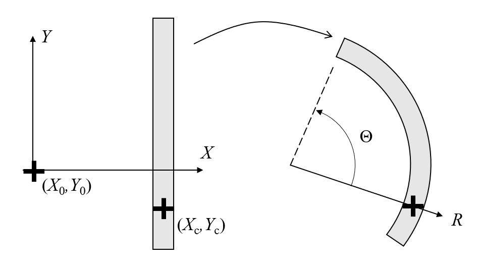
Wrapping a part about an axis involves defining a mapping between every point in the Cartesian undeformed state to the cylindrical deformed state.
To define this mapping, it is simplest to keep the CAD part aligned with the global Cartesian coordinate system such that the X-axis corresponds to the radial direction in the wrapped state. Next, define a point (X_0,Y_0) that the part will be wrapped around, as well as a point (X_c,Y_c) on the part that is pinned in space. The distance between these points is R_0. Then, consider a cylindrical coordinate system centered at the same origin point, with its R-axis pointing between the same two points. Choosing a point (X_c,Y_c) that is in the center of the part (assuming uniform thickness) implies that wrapping the part will not change the volume, but other points could be chosen, if a stretching or compression of the domain is desired. For example, choosing a point that lies on the surface of the part would mean that that surface does not change area.
To define this deformation, define a set of expressions that maps points in the XY-plane to points in the R \Theta-plane.
From these, the deformation expressions are:
These deformation expressions can be used directly within the Prescribed Deformation feature of the Moving Mesh or Deformed Geometry interfaces. For the case of wrapping about an arbitrary axis, a full three-dimensional rotation matrix needs to be constructed. Defining arbitrary rotations is addressed in this Learning Center article. In practice, wrapping about a Cartesian axis is preferred whenever possible. The results of such a deformation are shown in the figure below, and further analysis can be done directly on this deformed state.
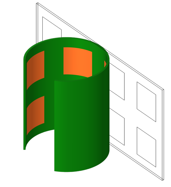
The deformed part after wrapping.
Meshing the Surrounding Domain via a Second Component and Mesh
Although deforming the part itself is interesting on its own, we often need to concern ourselves with the space around the part as well. For example, we may want to model the wrapped part within free space, a volume of complicated shape about the deformed part that is itself within another domain, such as a set of domains representing an infinite element or perfectly matched layer. An example of such a situation is shown in the image below of our wrapped part sitting within an empty, unmeshed, spherical space that has a meshed set of spherical layers about the outside.
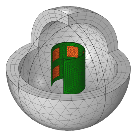
A wrapped part within an empty, unmeshed, spherical space and a meshed spherical layer of elements about the outside.
As we can see, there are two issues:
- The wrapped part now has a deformed mesh
- There is no mesh in the immediately surrounding space
We would like to remesh this wrapped part and introduce a mesh in the neighboring domain. The first step is quite easy: We simply have to remesh the deformed configuration, which then gives us a second mesh within our first Component in our model.
Next, we have to introduce a second component into our model, and within the Mesh branch of that second Component, we import the remeshed state from the first Component. This copies the mesh and allows us to introduce additional mesh operations. We need to add just two additional features. First, a Create Domains feature will create domains out of all fully enclosed regions of free space, such as the space between our wrapped part and the outside layer. Second, we add a Free Tetrahedral feature, which meshes the domain we just created: the volume between the wrapped part and the encapsulating shell. This mesh can now be used for any further analysis within the second Component of the model.

The mesh based upon the deformed configuration from the first component is imported into the second component within the model. The surrounding free space about the part can be defined as a domain and meshed.
Closing Remarks on Wrapping and Warping Geometries
We’ve introduced a method for taking a CAD part and wrapping it about an axis via an explicit deformation. We’ve also introduced a way of easily meshing the space around the deformed part and using this for further analysis. It is worth remarking that this remeshing approach will also work when the deformation of the solid is computed, rather than prescribed. In cases where a simple wrapping is desired, though, the approach shown here is much simpler. More complex deformed shapes can also be prescribed, as long as a mapping between the undeformed and deformed state can be defined.
The model demonstrating this technique is available via the button below:


Comments (4)
Ivar KJELBERG
September 12, 2021Hello Walter,
As usual thanks for a great Blog, giving new hints on how to deal with highly deformed structures.
Nevertheless, I have a little comment, for structural, if the strip is made of different materials it might not have a homogeneous stiffness, such that a fully regular shape would not be the “true final shape” if the part is rolled. And the stress buildup by rolling it (applying a pure torque on the lateral edges) would be somewhat different from the regularly rolled prescribed deformation solution.
As the stress buildup in the final “rolled” state might be of importance for fatigue or general lifetime analysis, one might need here to perform this is several steps, i.e. first to “prescribe” roll the part as you describe it, then to block the edges and leave the part to relax and find its own neutral position, and continue from thereon.
Anyhow great hint, and I see you seem to have a new (for me, only ?) “Learning Center Resources” web side referenced here, great, but I could not find its general entry point on your Web Learning Centre web page, probably its “to come”.
Sincerely
Ivar
Walter Frei
September 13, 2021 COMSOL EmployeeHello Ivar,
Thank you for the comments.
I should emphasize more strongly that this method can also be used in conjunction with Solid Mechanics. That is, one could solve for the deformed state of the solid part (which might include wrinkling, stress concentrations, etc… ) and then use that deformed state in the second part of the analysis.
However, setting up and solving such a highly nonlinear structural problem (it will involve geometric, material, and even possibly contact nonlinearities, and one would need to know exactly how the forces are applied during the fabrication process, to say nothing of the complexity introduced by gluing or adhesives) can be quite time-consuming, even for an experienced structural analyst.
Sometimes we just want to perform an electrical (or even other physics) analysis on the presumed deformed state, even if the deformed state being imposed by this technique is not precisely correct. And do keep in mind that we could introduce more complicated expressions (https://www.comsol.com/blogs/how-to-generate-random-surfaces-in-comsol-multiphysics/) if we wanted to see the effect of random deviations, or known variations, from an ideal curved shape as we’ve done here. It is that use-case which is being addressed here.
Thank you again for your feedback, and do keep an eye out for more upcoming resources!
Best Regards,
Walter
Simon
September 1, 2022Hello Walter,
Very helpful blog post, helped me to curve a geometry on itself, thank you !
However, in the formula of θ which is : “θ=(Y-Yc)/R0+atan2(Yc-Y0,Xc-X0)” I understand the part “atan2(Yc-Y0,Xc-X0)” which is basically the angle between our point and the x axis but why do we have to add “(Y-Yc)/R0” to it ? I do not get what that part of the formula represents.
Same question for the calcul of R which is : “(X-Xc)+R0” I understand we need R0 the distance to the origin for cylindrical coordinate system but why do we have to add “(X-Xc)” to it ?
Thanks,
Sincerely,
Simon.
Walter Frei
September 1, 2022 COMSOL EmployeeThe spatial coordinates are (X,Y) and the point at the centerline of the deformed part is (X_c, Y_c), we want to wrap such that the distance from (X_0, Y_0) to (X_c, Y_c) stays the same. All other distances ||(X-X_0, Y-Y0)|| will change.