Heat Transfer Module Updates
For users of the Heat Transfer Module, COMSOL Multiphysics® version 5.4 includes mixed diffuse-specular reflection and semitransparent surfaces for modeling surface-to-surface radiation, heat transfer in thin structures, and more capabilities for modeling radiation in participating media interfaces. Learn about these heat transfer features and more below.
Mixed Diffuse-Specular Reflections and Semitransparent Surfaces
A new algorithm for view factor computations, based on a ray-shooting method, can handle mixed diffuse-specular reflections as well as reflections and transmissions through semitransparent surfaces. Rough surfaces tend to reflect incident rays randomly in all directions regardless of incident direction, known as diffuse reflections. Smooth, mirror-like surfaces tend to reflect incoming rays according to the law of reflection where the angle of incidence is equal to the angle of reflection, known as specular reflection. The new capability for handling a mixture of diffuse and specular reflections can be used to create realistic and accurate models of a wide range of surfaces. The new ray-shooting method can also be used for modeling semitransparent surfaces that are not fully opaque, but instead transmit a fraction of the incident irradiation, for example, window glass. You can find this functionality used in the Surface-to-Surface Radiation with Specular Reflection model.
Incident irradiation induced by a radiation nonfocused beam bouncing on the two sides of a channel (left). The different configurations correspond to different surface properties, from a nearly ideal specular surface to a pure diffuse surface. For highly specular surfaces, the beam is reflected multiple times before it vanishes, while it is immediately damped for pure diffuse surfaces. The sketch on the right represents a similar case for a perfectly focused beam on specular surfaces.
Heat Transfer in Thin, Layered Structures
The functionality for heat transfer in thin structures has been dramatically expanded with a new set of powerful tools for modeling layered shells. Layered structures are defined using a new Layered Material feature that includes load/save of layered structure configurations from/to a file, a Layer Cross Section Preview feature, and a Layer Stack Preview feature. Each layer is assigned a material property, intrinsic rotation, thickness, and finite element discretization settings. In addition, the interfaces between each thin layer can be assigned separate interface properties. Optional tools for lumped modeling methodology are available for reducing the computational cost for both thermally thin or thermally thick structures. A new Layered Material dataset makes it possible to visualize results in thin, layered structures as if they were originally modeled as 3D solids.
The new functionality is available in all the heat transfer interfaces that include functionality for analyzing shells, thin layers, thin films, and fractures. When combined with the AC/DC Module, new multiphysics coupling features enable the modeling of electromagnetic heating and the thermoelectric effect in layered structures. When combined with the Composite Materials Module, a new multiphysics feature makes it possible to model thermal expansion in layered structures.
You can see this functionality used in the following models:
- aluminum_extrusion_fsi
- double_pipe_heat_exchanger
- finned_pipe
- electronic_enclosure_cooling
- heating_circuit
- parasol_and_solar_irradiation
- shell_and_tube_heat_exchanger
- surface_mount_package
- vacuum_flask_llmatlab
- disk_stack_heat_sink
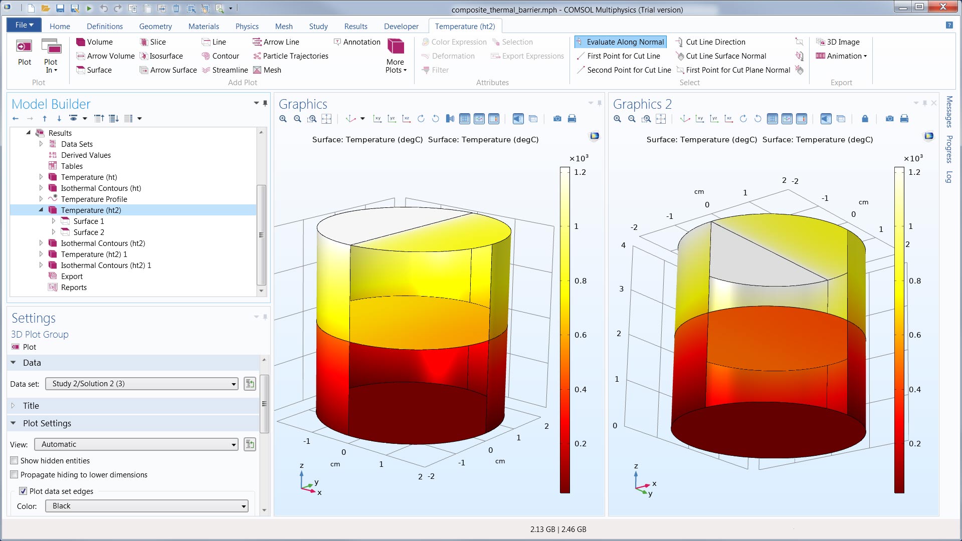
- composite_thermal_barrier (New)
- copper_layer
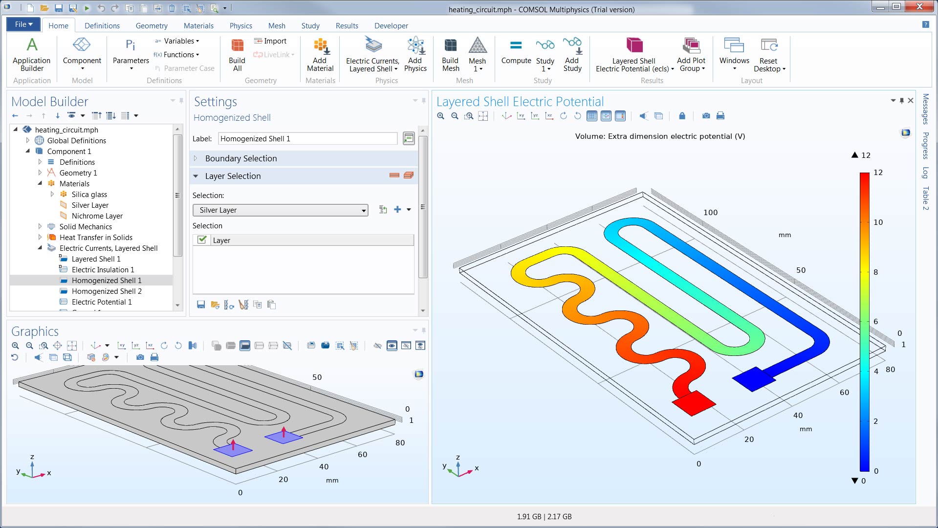 This multiphysics model of a heating circuit is defined using the new capabilities for thin, layered materials with a combination of heat transfer, electric currents, and structural membrane physics.
Extended Capabilities for Radiation in Participating Media
Important improvements have been made to the Radiation in Participating Media interface. A new option is available to control the nature of radiation scattering in semitransparent materials. The scattering characteristics are defined by the so-called Henyey-Greenstein phase function. In addition, several new quadrature options are available, and you can control the number of discrete ordinates, from 8 to 512, thus enabling detailed control of the trade-off between accuracy and computation speed. You can see this functionality used in the Radiative Cooling of a Glass Plate model.
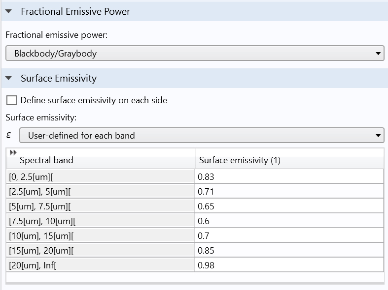
Surface-to-Surface Radiation with Wavelength-Dependent Material Properties
The Surface-to-Surface Radiation interface now supports an arbitrary number of spectral bands to model wavelength-dependent material properties. In addition, the user interface has been redesigned to improve usability when multiple spectral bands are used. Using multiple spectral bands, it is possible to define material properties such as the surface emissivity from a wavelength-dependent function or from a table, with one value per spectral band. A precise description of the wavelength-dependent surface properties increases the accuracy of simulation for scenarios like radiative cooling. You can see this functionality used in the Sun's Radiation Effect on Two Coolers Placed Under a Parasol model.
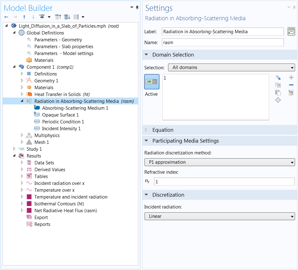
Radiation in Absorbing-Scattering Media Interface — Light Diffusion Equation
The new Radiation in Absorbing-Scattering Media interface is available for modeling propagation, absorption, and scattering of radiation in a semitransparent medium. In particular, it is well suited for modeling light diffusion in a nonemitting medium. Similarly to the Radiation in Participating Media interface, it solves the radiative transfer equation, but with no emission term. Therefore, the two interfaces share the same discretization methods (P1 approximation and discrete ordinates method) and options for scattering. When the P1 approximation is used, the solved equation is known as the light-diffusion equation. You can see this functionality used in the Light Diffusion in a Slab of Particles model.
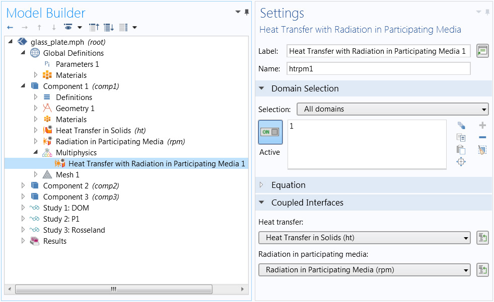
Multiphysics Couplings for Heat Transfer with Radiation
In previous versions, the Surface-to-Surface Radiation and Radiation in Participating Media features were available as options in all heat transfer interfaces, as well as in separate standalone interfaces. In COMSOL Multiphysics® version 5.4, they are only available as standalone interfaces, and can be coupled with any relevant heat transfer interfaces using new multiphysics interfaces. This new modeling approach simplifies model management in the Model Builder.
Refactoring of Functionalities into Subnodes
For a better user experience, a number of feature subnodes have been added to the heat transfer interfaces. They are used to modify the configuration of their respective parent feature. In future versions, the following subnodes will replace the corresponding main features:
- The Phase Change Material subnode replaces the Phase Change Material feature for fluids, extends its capabilities to solids and porous media, and implements the apparent heat capacity formulation for modeling phase change
- The Convectively Enhanced Conductivity subfeature is available under the Fluid and Moist Air nodes, and accounts for the convective heat flux by enhancing the fluid thermal conductivity according to the Nusselt number
- The Thermal Damage subnode is available under the Biological Tissue node to define the damage model
- The Optically Thick Participating Medium subnode, available in the heat transfer interfaces, accounts for the Rosseland approximation for radiative heat transfer in media with high optical thickness, and provides the settings needed to account for the radiative effects by enhancing the thermal conductivity
You can see these new features used in the following models:
- continuous_casting
- cooling_solidification_metal
- isothermal_box
- glass_plate
- conical_dielectric_probe
- microwave_cancer_therapy
- tumor_ablation
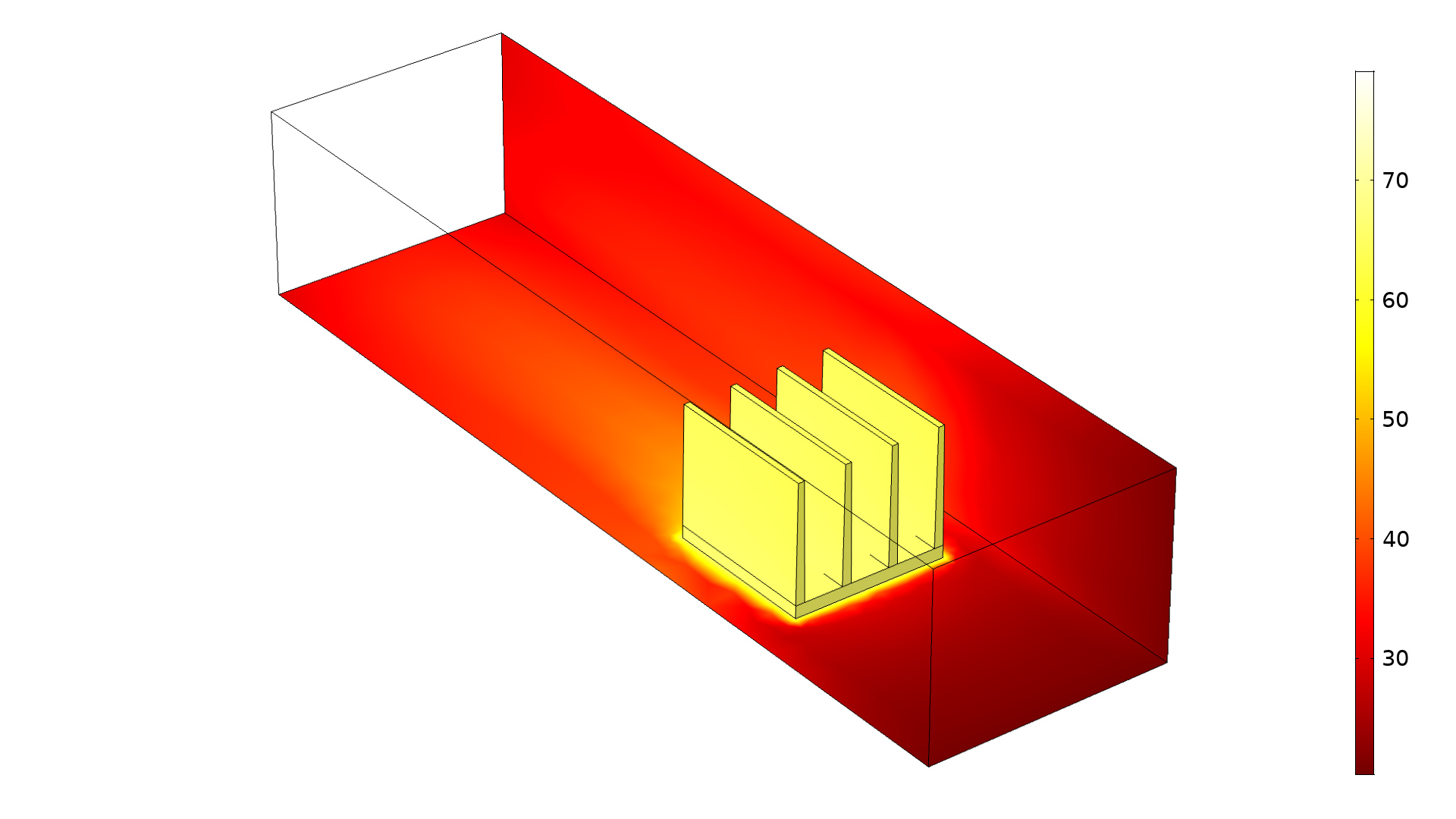
Temperature distribution in an isothermal box aimed at transporting refrigerated articles. A phase-change material is modeled using a Fluid feature with the Phase Change Material subfeature.
Heat and Moisture Flow Multiphysics Interface
A set of new Heat and Moisture Flow multiphysics interfaces are available under the Heat Transfer > Heat and Moisture Transport branch to couple heat transfer and moisture transport in air by laminar and turbulent flows. The different interfaces couple the laminar and turbulent versions of the single-phase flow interfaces with the Heat Transfer in Moist Air and Moisture Transport in Air interfaces. The Heat and Moisture, Moisture Flow, and Nonisothermal Flow multiphysics coupling nodes handle turbulent mixing as well as heat and moisture wall functions for turbulent flows, and account for temperature and moisture content dependency of material properties in the fluid flow equations in air.
The evaporative cooling model combines single-phase flow with the Heat Transfer in Moist Air and Moisture Transport in Air interfaces.
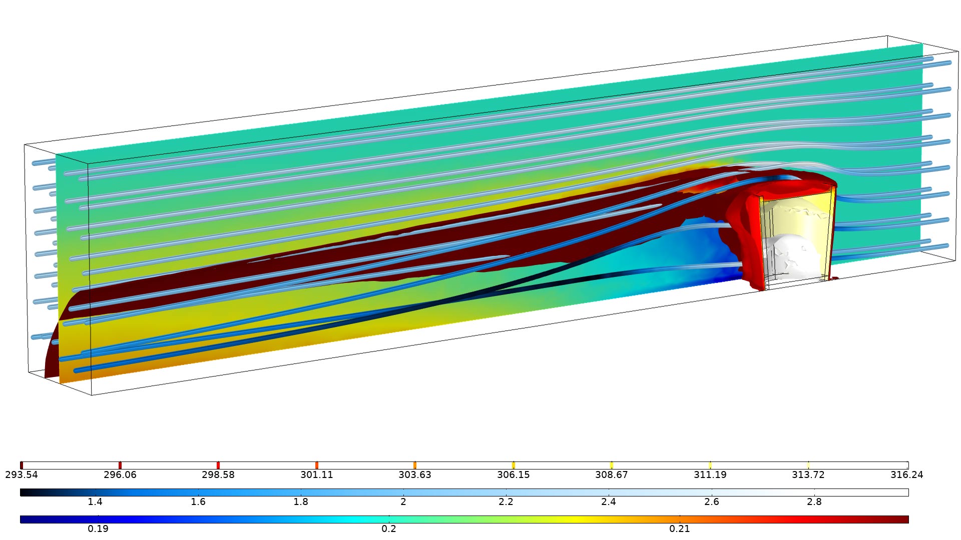
Heat Transfer in Solids and Fluids Interface
The new Heat Transfer in Solids and Fluids interface replaces the heat transfer interface that was previously available exclusively in the Conjugate Heat Transfer multiphysics interface. It has a Solid feature, activated by default on all domains, and a Fluid feature, with an empty selection by default. The settings are optimized for conjugate heat transfer modeling. Use this interface as you plan to build a model incrementally starting from heat transfer only and introducing flow as a second step. This is illustrated in the chip_cooling example of the Introduction to the Heat Transfer Module PDF.
You can also find this functionality in the following models:
 Temperature profile in the chip cooling tutorial. The accuracy of the model is gradually improved by adding more features in a sequence of steps. Starting from a model that includes only heat transfer in solids, the model is then expanded to include fluid flow and finally surface-to-surface radiation.
Perfectly Insulating Interior Walls
The Thermal Insulation feature is now available on interior boundaries, and it can be used to model thin materials between fluid domains as perfect insulators. The resulting temperature field is discontinuous across such boundaries. You can see this functionality used in the Thermal Insulation on Internal Boundary model.
Ambient Thermal Properties
Ambient properties can be defined from an Ambient Thermal Properties node under Definitions. It contains the Ambient Settings section that was previously available in the Heat Transfer interface. Several Ambient Thermal Properties nodes may be added in a single model. This makes it possible to use ambient properties when no heat transfer interface is present in a model.
In addition, the surface-to-surface interface has been improved so that it is possible to define the solar position by using Ambient Thermal Properties including the date and position of the selected weather station.

A model containing an Ambient Thermal Properties node that defines time-dependent ambient properties. The graph shows the ambient temperature and relative humidity over the two days for which the simulation is run.
Default Solver Settings
There are numerous improvements to the default solver settings for heat transfer. For large nonisothermal flow models, the default multigrid preconditioner settings have been updated with more robust settings that will give computational speedup in some cases. Furthermore, the models containing a Local Thermal Non-Equilibrium coupling now always solve for the coupled two-temperature field variables with better and faster convergence. Accordingly, all models with the Nonisothermal Flow coupling feature have been updated.
Improved Default Plots for Temperature Discontinuities
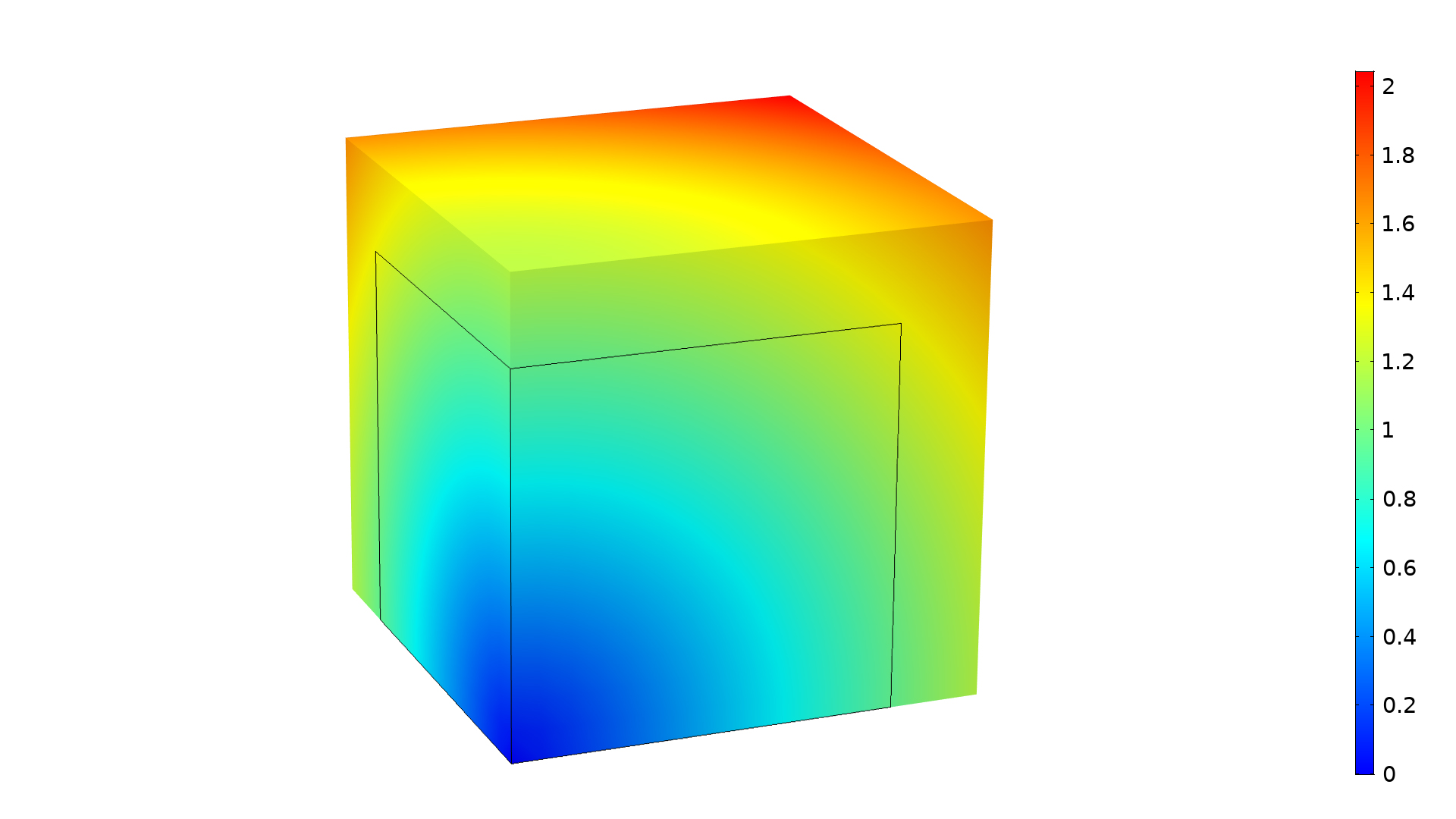
Additional surface plots are generated by default in the Temperature plot group of 3D models when the Thermal Contact or Thermal Insulation features are active on interior boundaries. This displays the different temperatures on both sides of such boundaries.
 The temperature field seen from two different angles. Since the temperature is discontinuous across the central boundary, the temperature shows different values on the two sides.
New Tutorial Models
COMSOL Multiphysics® version 5.4 brings several new tutorial models.
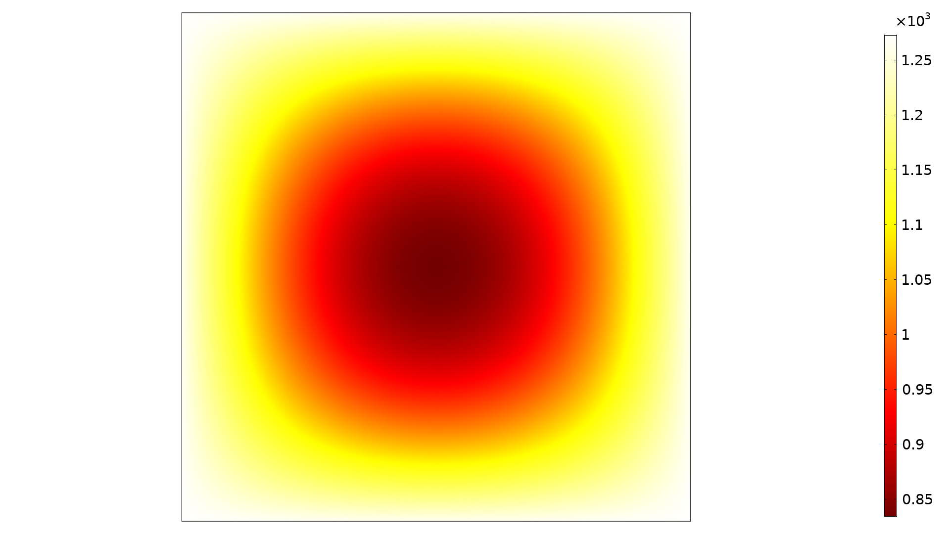
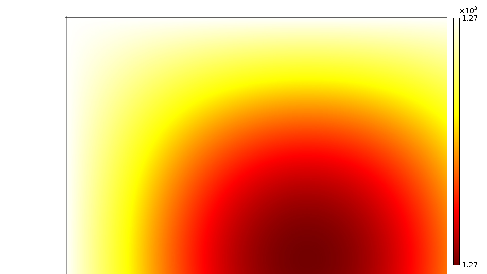
Isothermal Box

Temperature distribution in an isothermal box aimed at transporting refrigerated articles. A phase-change material is modeled using a Fluid feature with the Phase Change Material subfeature.
Search in the Application Library:
isothermal_box
Action on Structures Exposed to Fire — Thermal Stress in a Beam
 Thermal stress in a beam exposed to a temperature gradient with highly nonlinear material properties. The results are compared to reference values from the European Standard DIN EN 1991-1-2.
Search in the Application Library:
fire_effects_beam
Action on Structures Exposed to Fire — Cooling Process
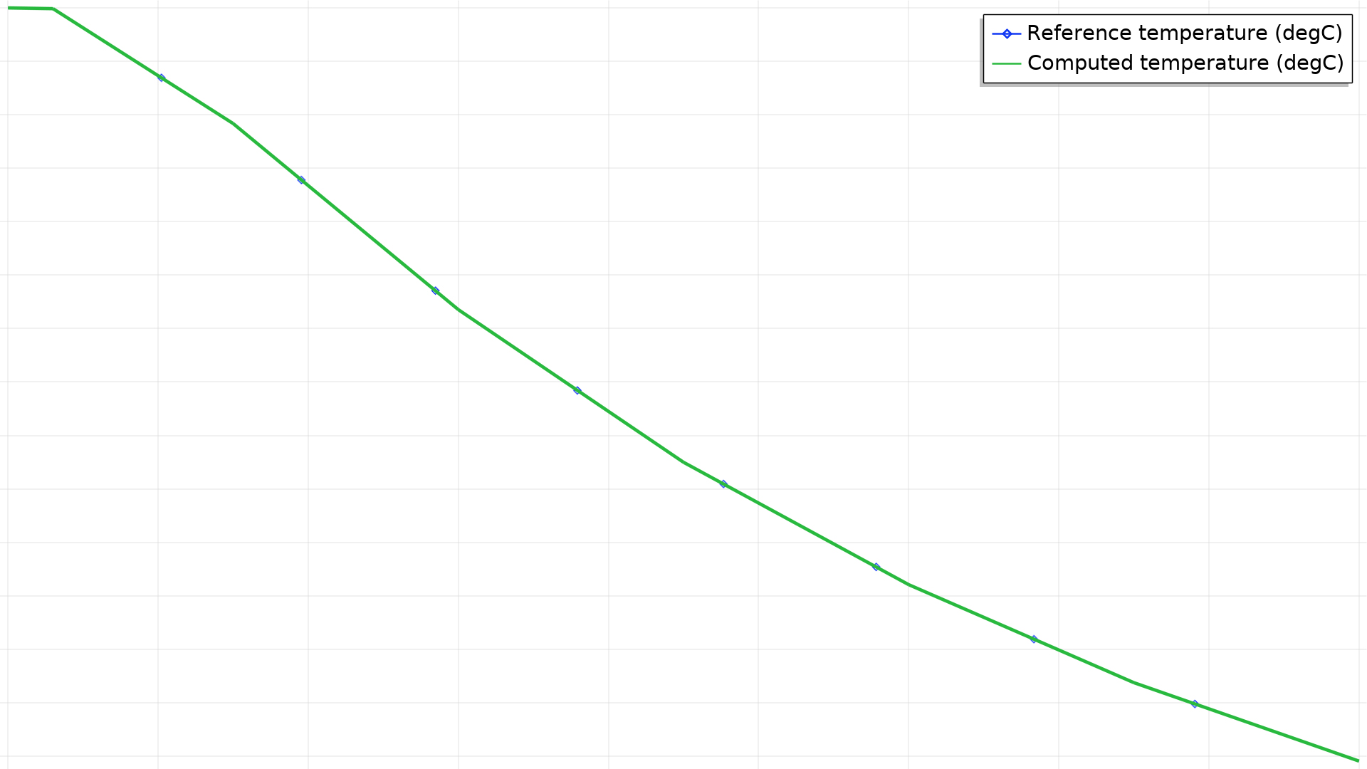 Temperature variation due to a convective cooling process. The results are compared to reference values from the European Standard DIN EN 1991-1-2.
Search in the Application Library:
fire_effects_cooling
Action on Structures Exposed to Fire — Heating Process
 Temperature profile for a heating process due to convection and radiation using a temperature-dependent thermal conductivity. The results are compared to reference values from the European Standard DIN EN 1991-1-2.
Search in the Application Library:
fire_effects_heating
Action on Structures Exposed to Fire — Heat Transfer in Multiple Layers
 Temperature profile through layers with different thermal properties, inspired by heat transfer through a hollow steel section with filling. The results are compared to reference values from the European Standard DIN EN 1991-1-2.
Search in the Application Library:
fire_effects_multiple_layers
Action on Structures Exposed to Fire — Thermal Elongation
 Total displacement due to thermal expansion using a prescribed thermal strain function. The results are compared to reference values from the European Standard DIN EN 1991-1-2.
Search in the Application Library:
fire_effects_thermal_elongation
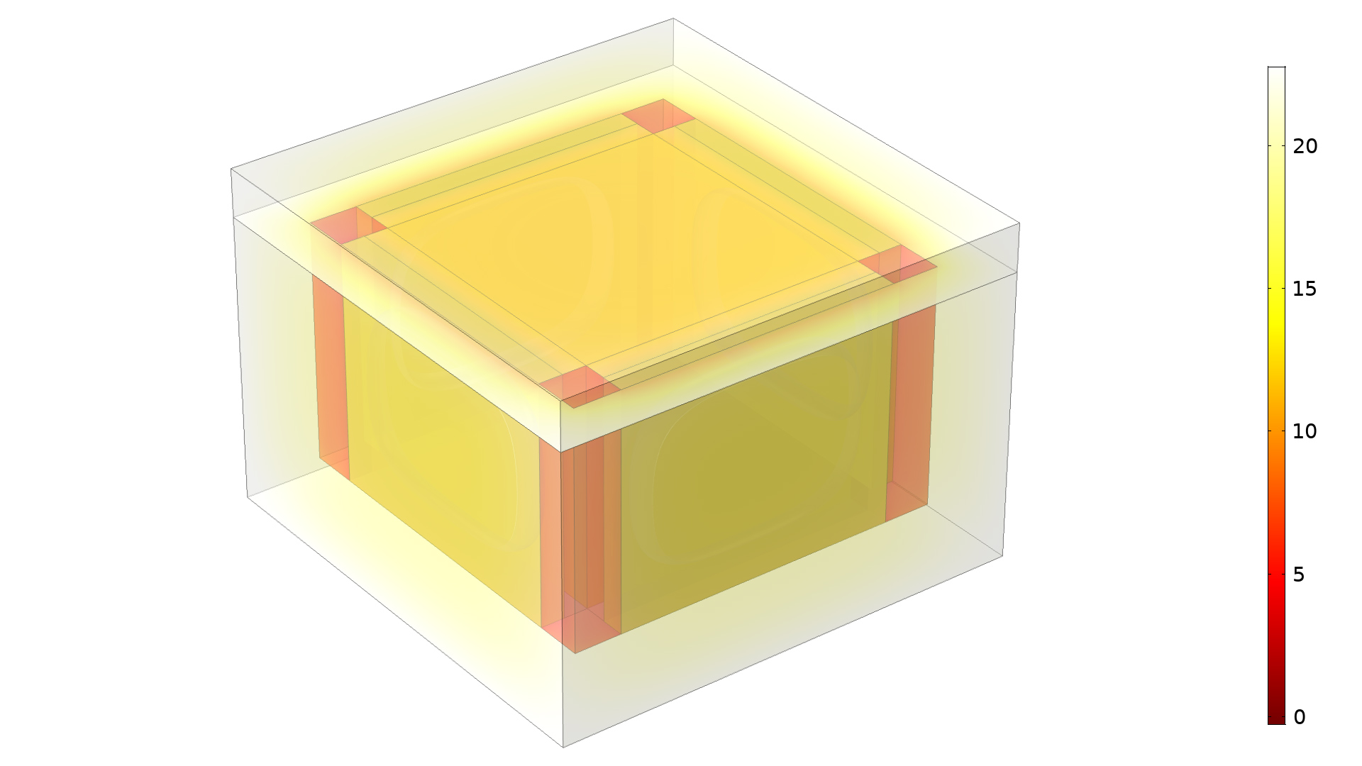
Heating Circuit
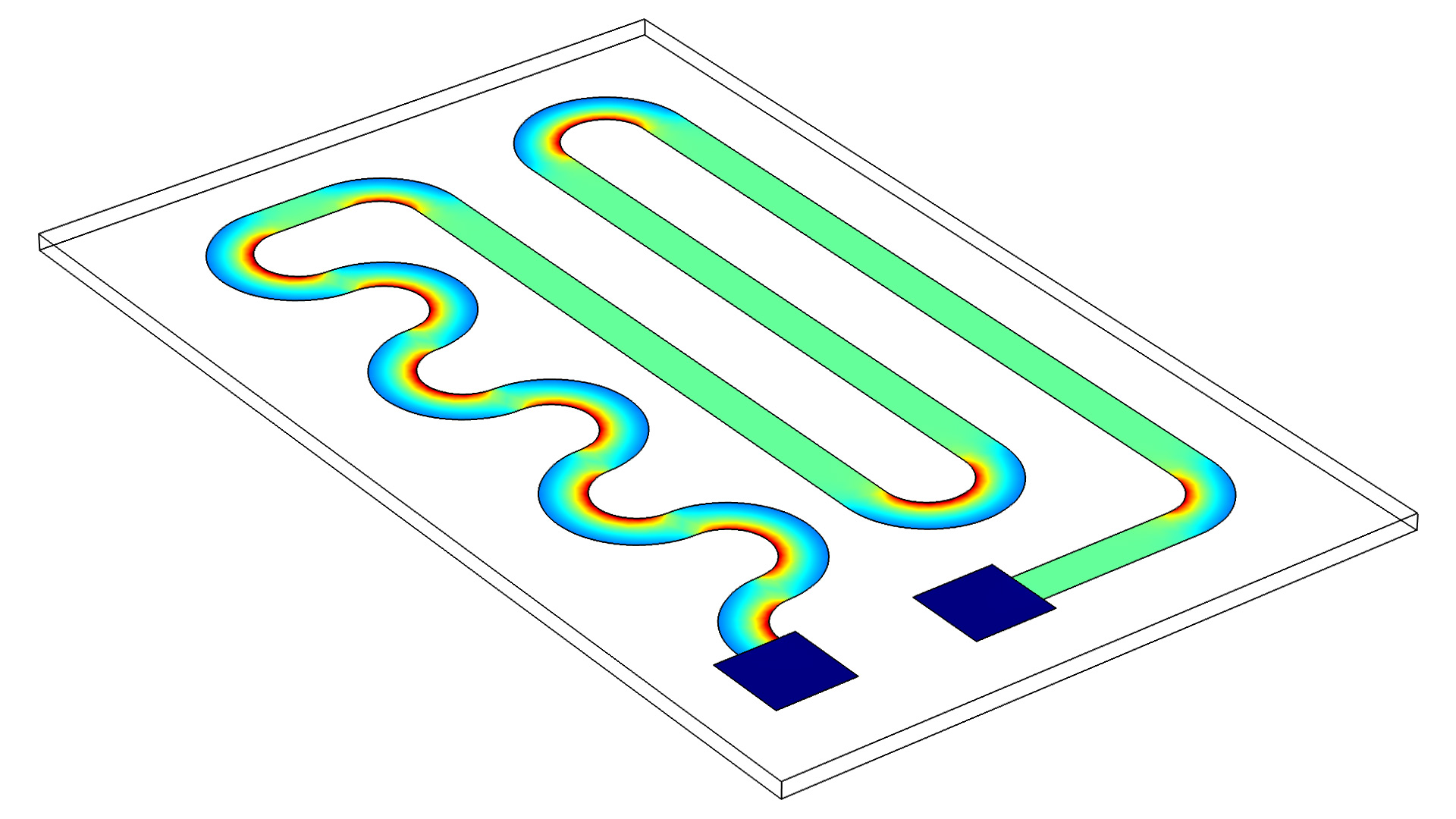 Heat generation in a resistive layer with a 12 V potential drop, modeled using the layered shells technology.
Search in the Application Library:
heating_circuit