COMSOL Multiphysics^® 6.2 Release Highlights

Acoustics Module Updates

For users of the Acoustics Module, COMSOL Multiphysics^® version 6.2 introduces a new frequency-dependent Impedance condition for time-domain pressure acoustics, a new anisotropic material model in the Poroelastic Waves interface, and a new Port boundary condition for enhanced modeling of aeroacoustics based on linearized potential flow. Learn about these updates and more below.

Frequency-Dependent Impedance Conditions in Time Domain

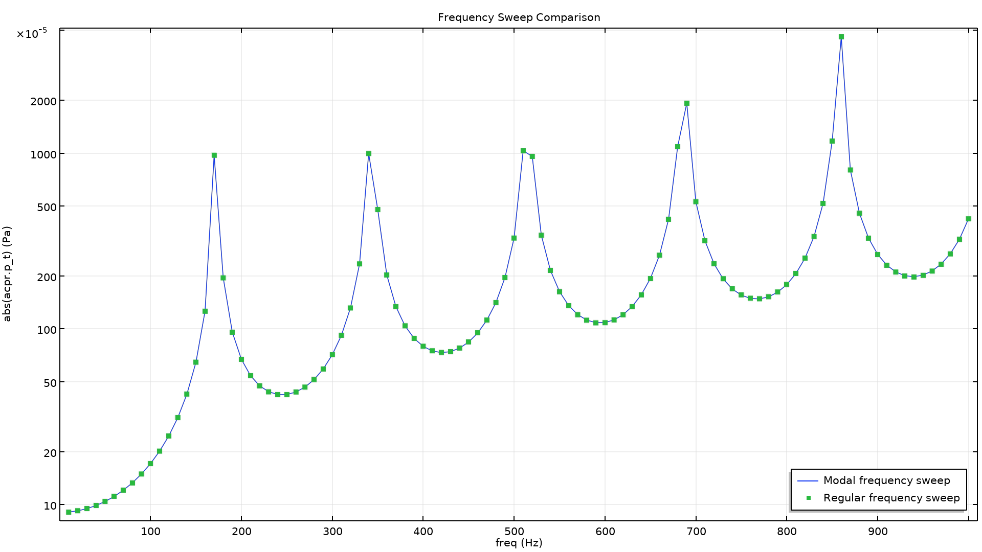
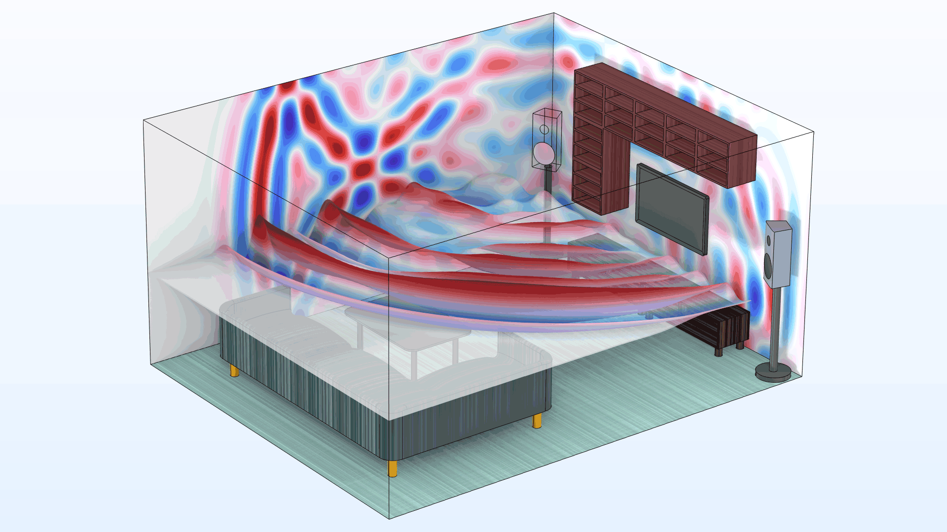
For the Pressure Acoustics, Transient interface and the Pressure Acoustics, Time Explicit interface, there is new functionality for specifying and setting up frequency-dependent impedance conditions in the time domain. The functionality provides a rational approximation of the frequency-domain data, resulting in a system of ordinary differential equations (memory equations for the inverse Fourier transform) solved in the time domain. A new function for fitting or interpolation has been added to perform the transformation from the frequency-domain data to the time domain, where the fitting relies on a variant of the adaptive Antoulas–Anderson (AAA) algorithm. This new functionality is showcased in the updated Wave-Based Time-Domain Room Acoustics with Frequency-Dependent Impedance tutorial model.

The Impedance boundary condition in the Pressure Acoustics, Transient and Pressure Acoustics, Time Explicit interfaces can now be used to model realistic surface properties, such as those of an absorbing panel or any other surface that has frequency-dependent absorbing properties. There are two new options available, Serial coupling RCL and General local reacting (rational approximation), the latter of which relies on a special transformation of the surface impedance data, which can be achieved with the new Partial Fraction Fit function. This new functionality is essential when modeling, for example, realistic wave-based room acoustics simulations in the time domain.

The Partial Fraction Fit function transforms frequency-domain data into a form that is suitable for a time-domain analysis. The function performs a rational approximation of frequency-domain responses. This makes it possible to compute the inverse Fourier transform analytically and thus obtain the time-domain impulse response function. The fitting algorithm can be used for any data, but it is particularly important and useful for surface impedance data in acoustics simulations.

The Impedance boundary condition in the Pressure Acoustics, Time Explicit interface. The necessary data for the General local reacting (rational approximation) condition is directly imported from the Partial Fraction Fit function that fits the frequency-domain admittance.

Anisotropic Poroelastic Material Model in the Poroelastic Waves Interface

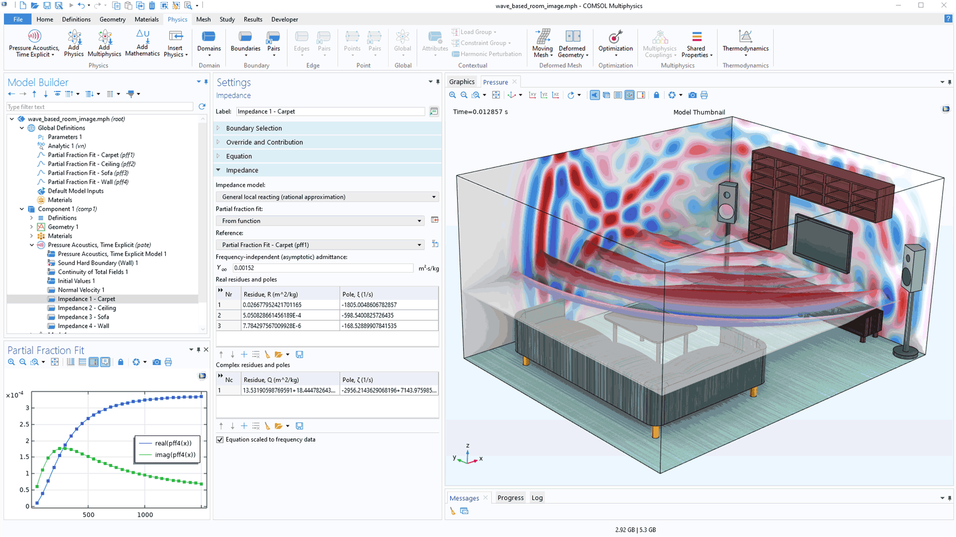
The Poroelastic Waves interface has been extended to include a new material model, Anisotropic Poroelastic Material. Many porous materials, like fibrous materials, exhibit anisotropic properties. The anisotropic properties can now be defined for the elastic matrix material properties as well as the relevant poroacoustic properties, i.e, the flow resistivity, the tortuosity factor, and the viscous characteristic length. You can view this material model in the new Transverse Isotropic Porous Layer tutorial model.

The Anisotropic Poroelastic Material model, where the porous matrix properties are anisotropic for the modeled fibrous material.

Restructured Poroelastic Waves Interface

The Poroelastic Waves interface has been restructured for an improved user experience. Features that apply to a porous elastic matrix and those applicable to saturating fluids are now located in separate menus. In addition, these features can be applied to the same boundary for defining a multitude of mixed conditions. The following tutorial models showcase this new update:

• transverse_isotropic_porous_layer
• reflections_water_sediment
• acoustics_particulate_filter

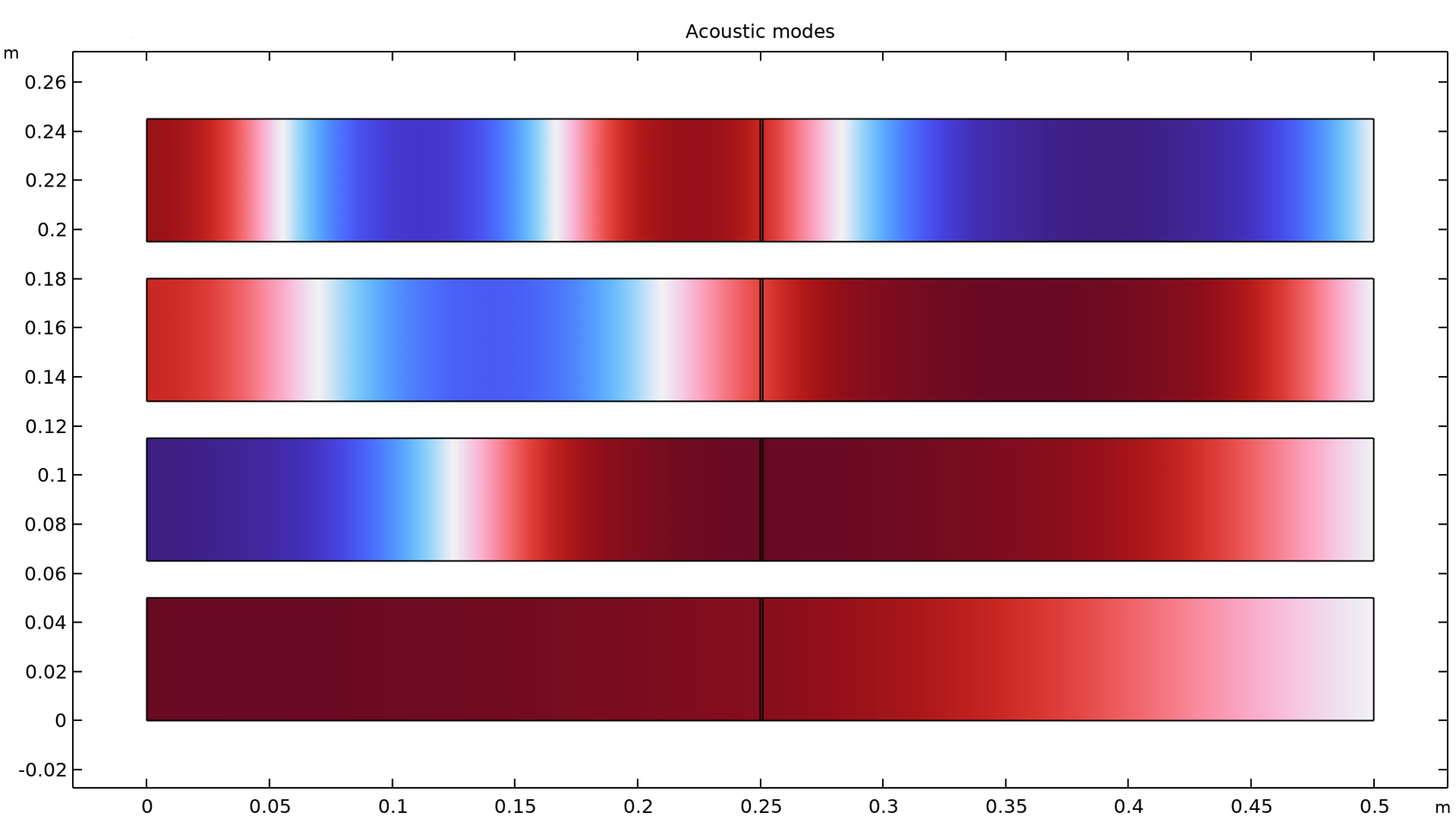
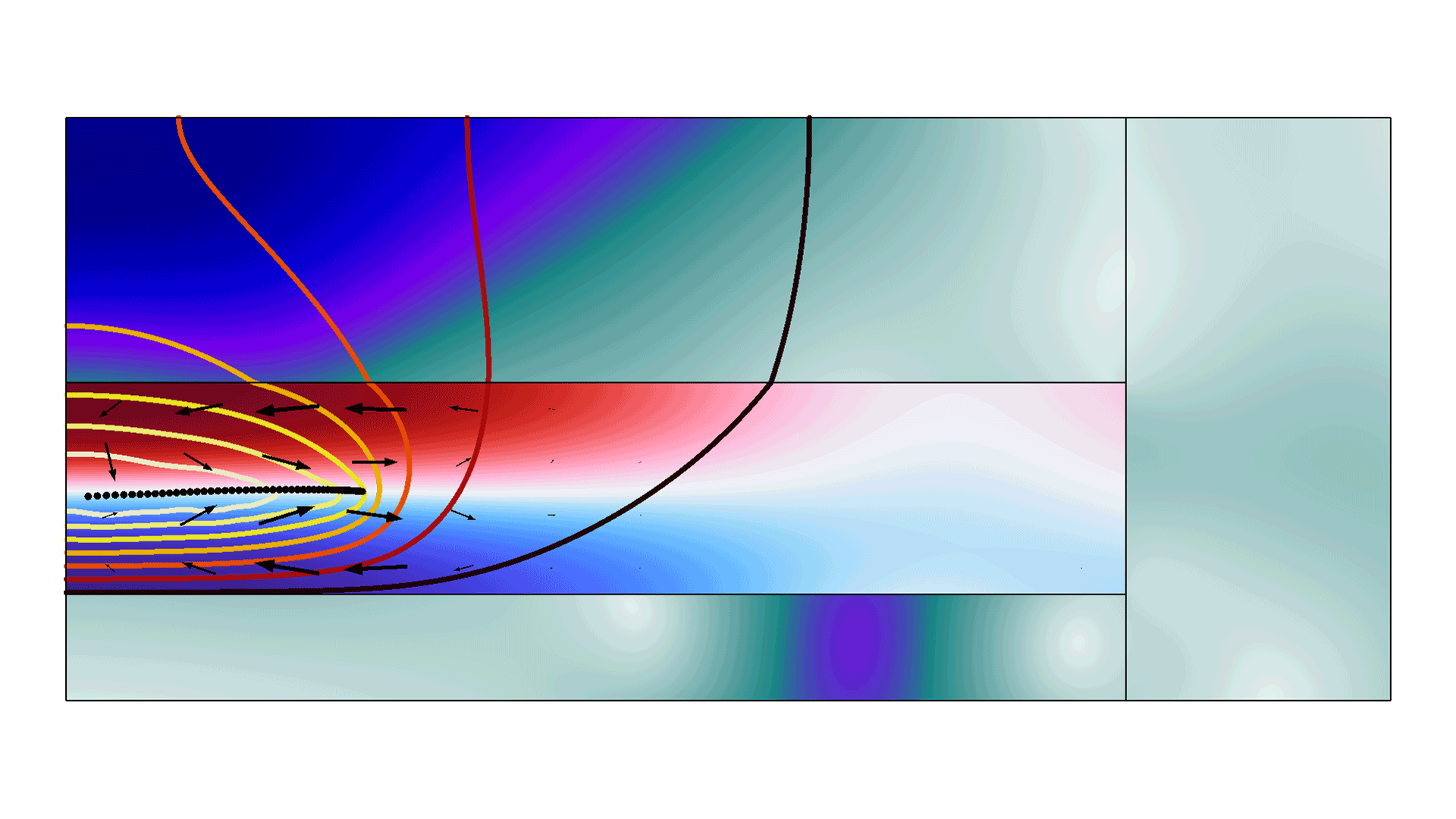
Port Condition for Linearized Potential Flow

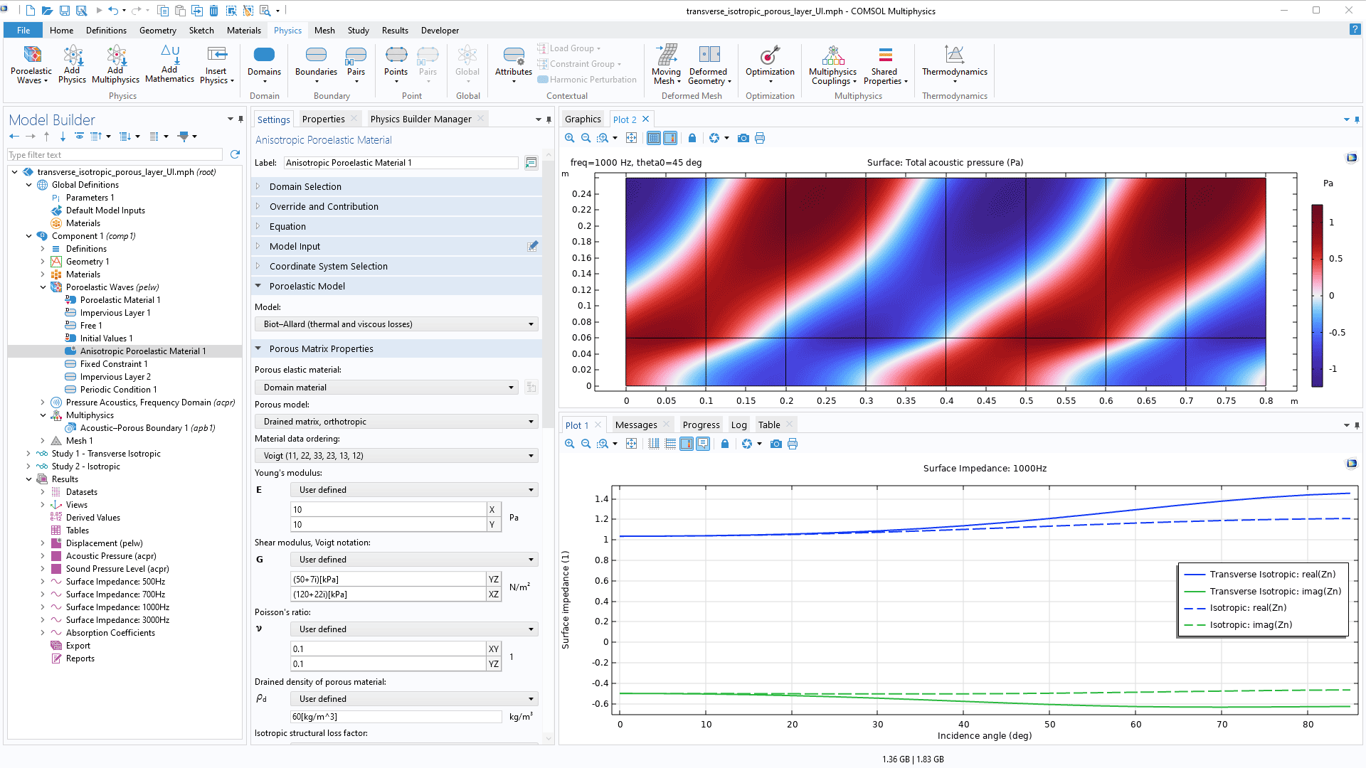
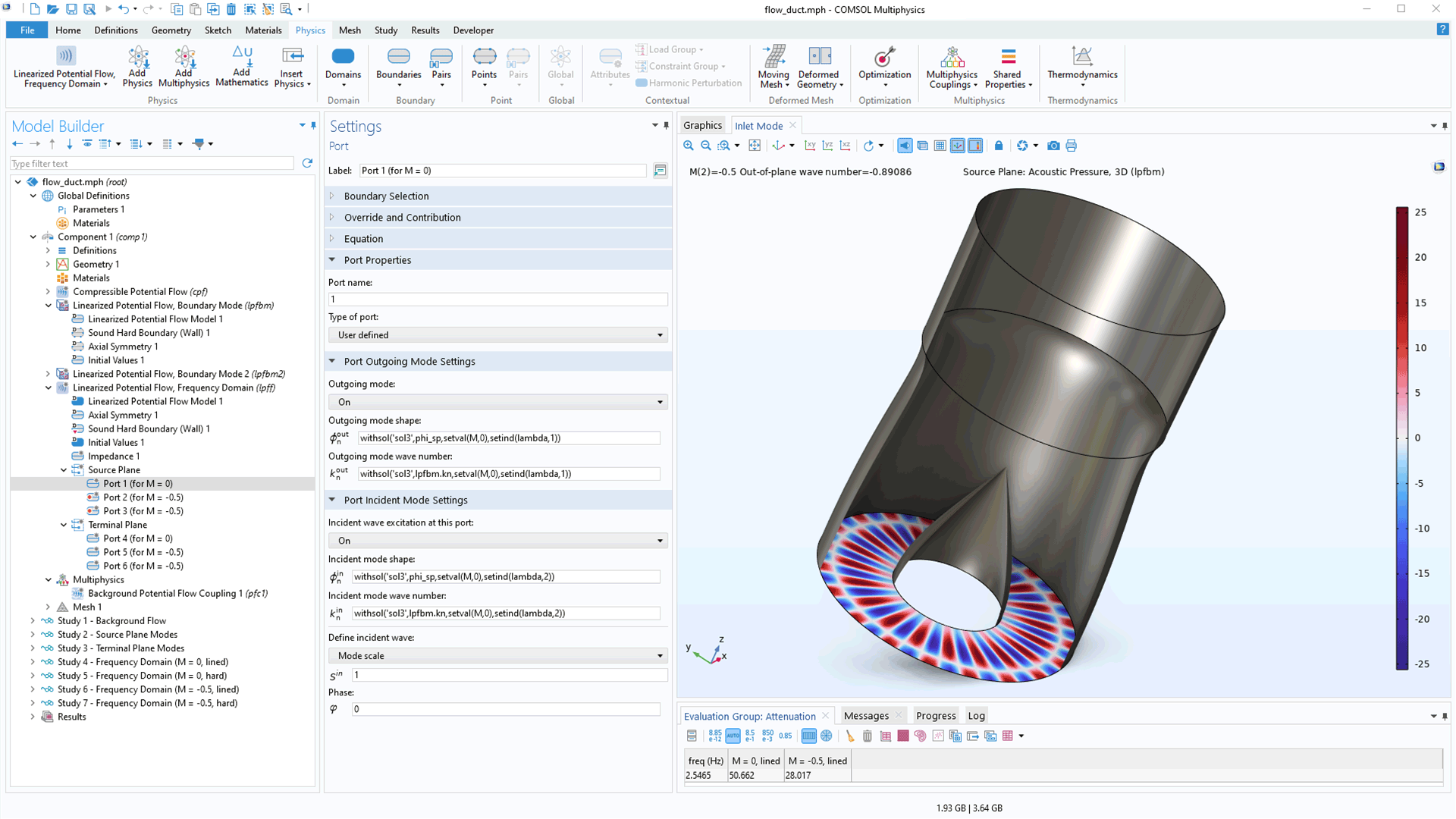
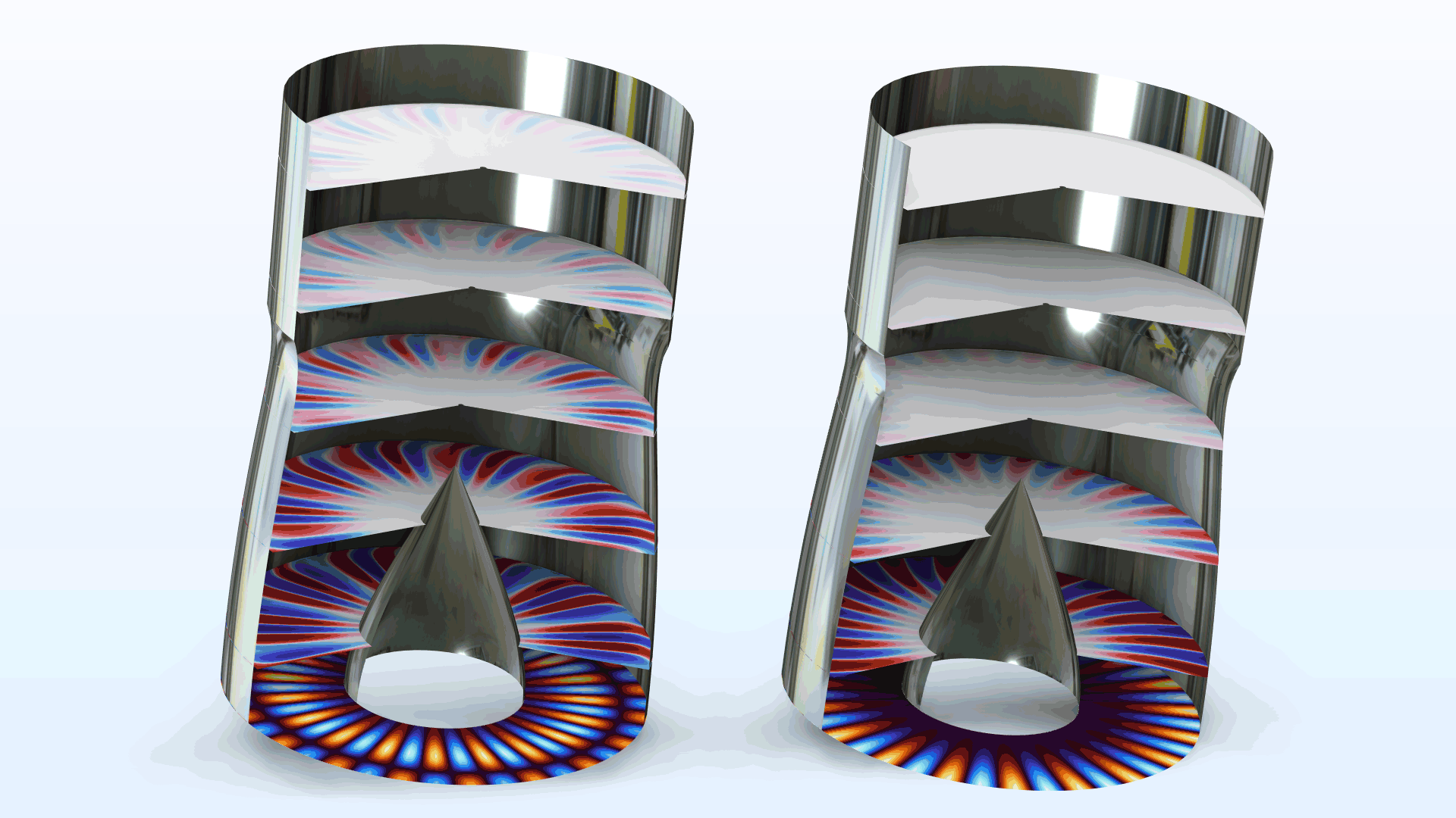
A Port boundary condition has been added to the Linearized Potential Flow interface. The Port condition is used to excite and absorb specific acoustic modes that enter or leave waveguide structures, such as a turbofan duct or other channel structures. This functionality is applicable to convected acoustics simulations based on the linearized potential flow formulation. To provide a complete acoustic description, several port conditions are applied to the same boundary to facilitate modal decomposition of noise sources. Within the studied frequency range, all relevant propagating modes can be accounted for. The Linearized Potential Flow, Boundary Mode interface is then used to analyze and identify the propagating and nonpropagating modes. You can see this new feature in the Flow Duct tutorial model.

The new Port boundary condition in the Linearized Potential Flow, Frequency Domain interface. Here, it is used to study the modal transmission of a turbojet engine flow duct.

Modal sound transmission simulation in a turbojet engine intake model. The results are taken from the Flow Duct tutorial model, in which the new Port boundary condition is used.

Impedance Condition in the Linearized Potential Flow, Boundary Mode Interface

The Impedance boundary condition can now be added to the Linearized Potential Flow, Boundary Mode interface when computing propagating and nonpropagating modes. It is useful to add this condition in combination with the Port boundary conditions in the Linearized Potential Flow, Frequency Domain interface when exciting a waveguide system with realistic outgoing and incident modes in lined waveguide configurations.

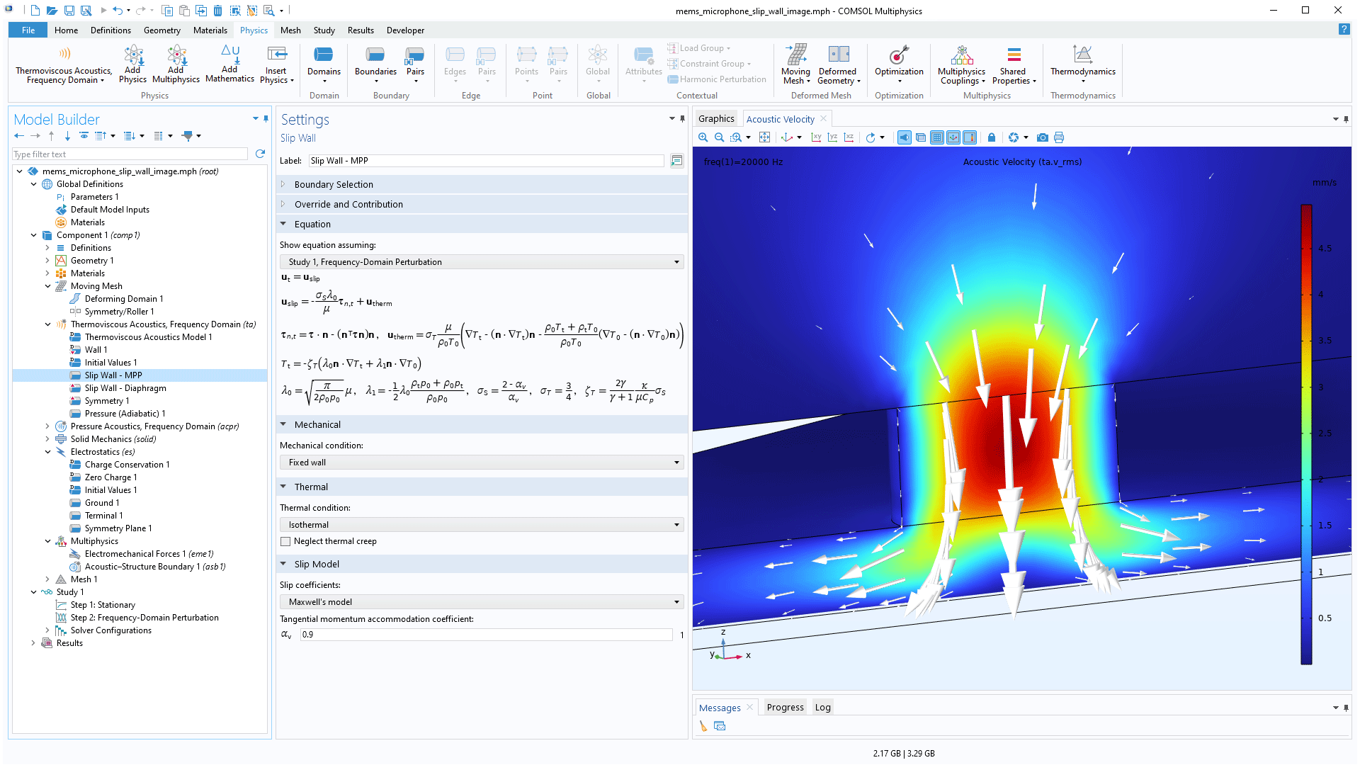
Slip Wall Feature in Thermoviscous Acoustics for Nonideal Wall Conditions

A new Slip Wall boundary condition is available for thermoviscous acoustics to model the effective nonideal wall conditions that exist in the slip flow regime, provided that the Knudsen number is in the range of 0.001 to 0.1. This condition is used for systems with very small geometrical dimensions or systems running at very low ambient pressures. This is relevant when modeling, for example, MEMS transducers and other microdevices, as seen in the MEMS Microphone with Slip Wall tutorial. To model a slip wall on an interior boundary, you can use the Interior Slip Wall condition. The new Slip Wall feature can be viewed in the Viscous Damping of a Microperforated Plate in the Slip Flow Regime tutorial model.

Use of the Slip Wall feature for modeling the damping properties of a microperforated plate (MPP). The Slip Wall condition is essential for modeling acoustics in MEMS devices.

Surface Tension Feature in Thermoviscous Acoustics

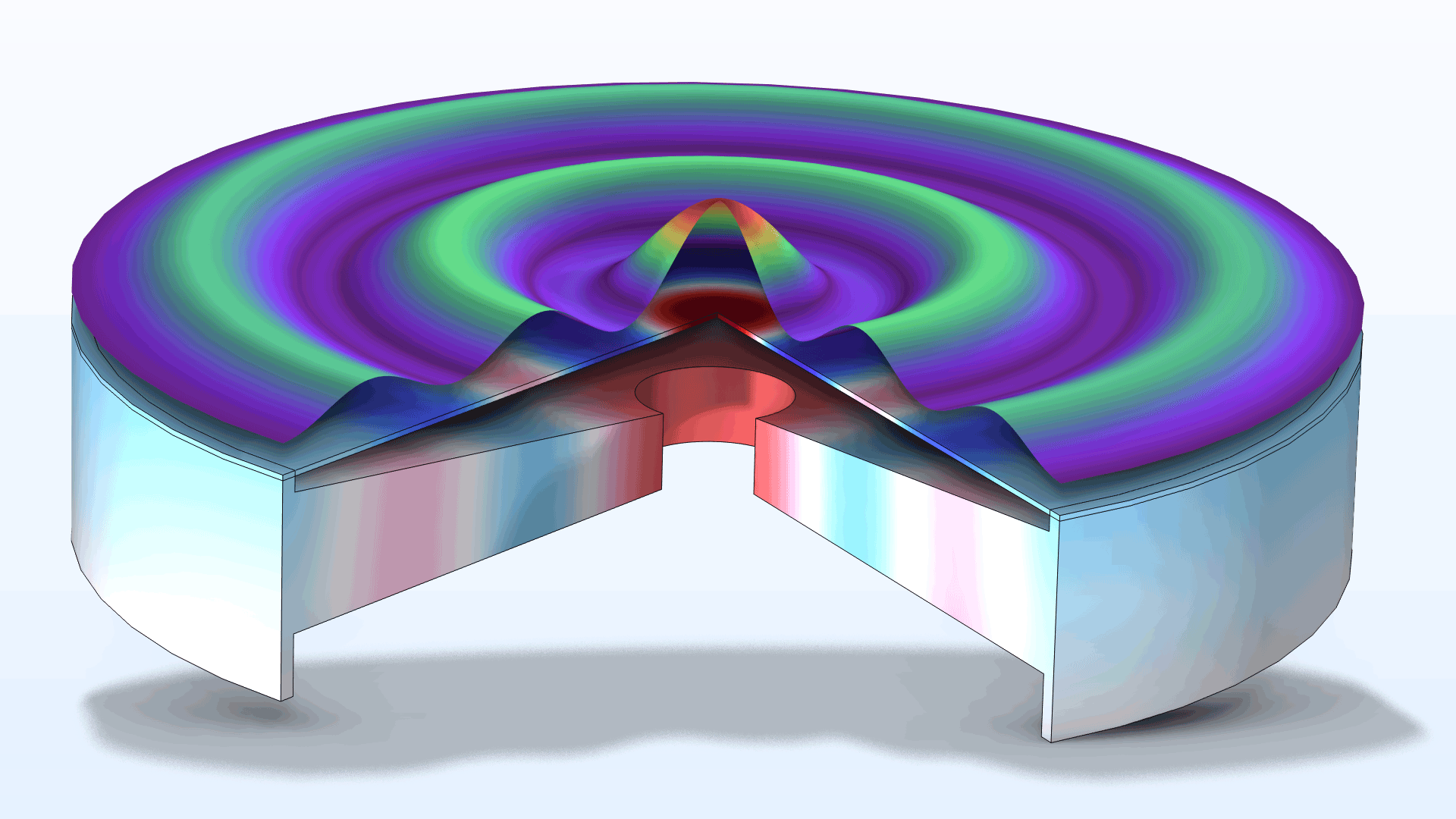
A new Surface Tension feature in the Thermoviscous Acoustics, Frequency Domain interface adds the necessary interior condition for modeling the interface between two fluids including surface tension effects. This acoustic (perturbation) formulation of the Young–Laplace equation relies on a linearization around the stationary shape of the fluid–fluid interface. This feature is important when modeling small, curved interfaces between two different immiscible fluids, like microbubbles or microdrops, in, for example, inkjet applications. The new Eigenmodes in Air Bubble with Surface Tension tutorial model showcases this feature.

New RCL Option for the Impedance in Thermoviscous Acoustics, Frequency Domain

An RCL option has been added to the Impedance boundary condition in the Thermoviscous Acoustics, Frequency Domain interface. This condition is useful for modeling the interaction between an acoustic field and simple spring–mass–damper systems using a lumped representation. For example, you can model acoustic–structure interactions with a microphone model using a lumped representation of the microphone's flexible membrane.

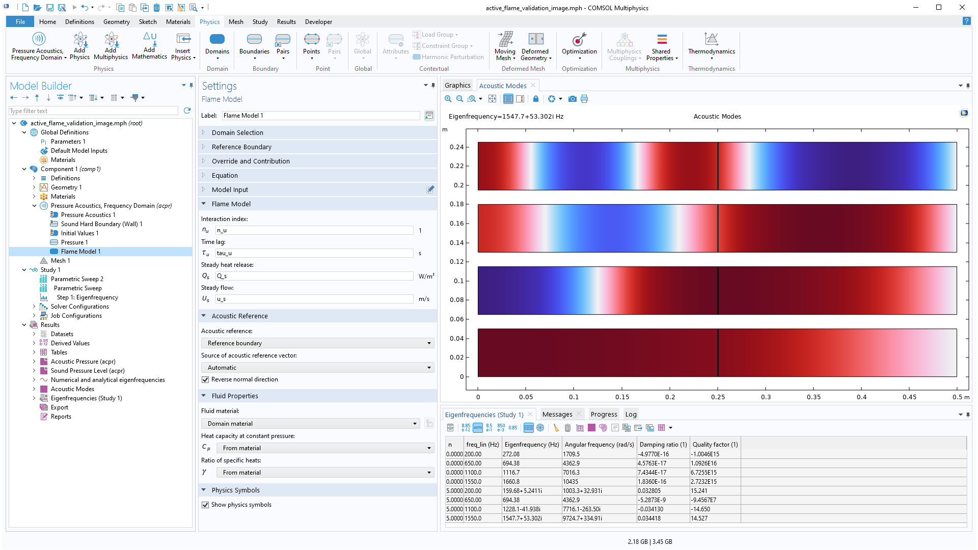
Flame Model in Pressure Acoustics, Frequency Domain

A new Flame Model feature in the Pressure Acoustics, Frequency Domain interface makes it possible to define a heat source using a flame model, typically for the stability analysis in a combustion setup. The heat source depends on the acoustic field and is defined in terms of the n-tau model. In combustion engines, the heat release depends on acoustic oscillations of the fresh fuel supply, and the acoustic oscillations are affected by the heat release. This may result in acoustic modes becoming either unstable or damped. View this feature in the new Active Flame Validation tutorial model.

The new Flame Model feature in the Pressure Acoustics, Frequency Domain interface.

New and Improved Multiphysics Couplings and Functionality

The Acoustic FEM–BEM Boundary coupling and the Acoustic–Structure Boundary coupling now include the option to add subfeatures, and two new multiphysics couplings have been added to the Acoustics Module to simplify the modeling workflow.

Acoustic–Thermoviscous Acoustic Boundary Multiphysics Coupling For Assemblies

A new boundary pair version of the previously available Acoustic–Thermoviscous Acoustic Boundary coupling has been added. This coupling is suited for modeling assemblies with nonconforming meshes.

New Thermoviscous Acoustic–Thermal Perturbation Boundary Multiphysics Coupling

A new Thermoviscous Acoustic–Thermal Perturbation Boundary multiphysics coupling has been added to couple the acoustic temperature variation in fluids with the temperature fluctuation in solids. This coupling acts as an interaction between either the Thermoviscous Acoustics, Frequency Domain interface or the Thermoviscous Acoustics, Transient interface and the Heat Transfer in Solids interface. This new coupling is useful, for example, for advanced acoustics simulations of thermoacoustic engines and pumps. You can see this functionality in the updated Thermoacoustic Engine and Heat Pump tutorial model.

Interior Impedance for the Acoustic FEM–BEM Boundary Multiphysics Coupling

When coupling pressure acoustics models based on the finite element method (FEM) and boundary element method (BEM) using the Acoustic FEM–BEM Boundary multiphysics coupling, an impedance subfeature can now be added between the two domains. This extends the use of the hybrid FEM–BEM modeling strategy, which is useful for large acoustical problems.

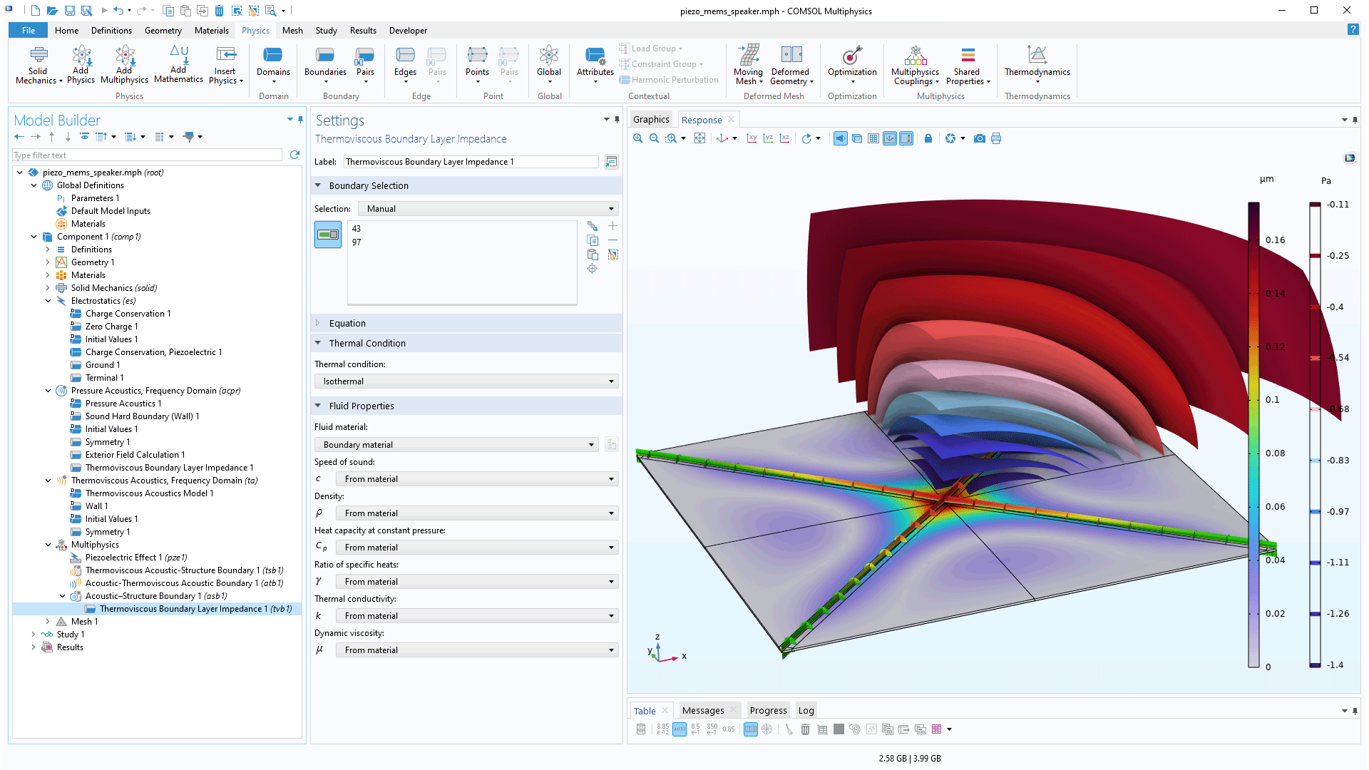
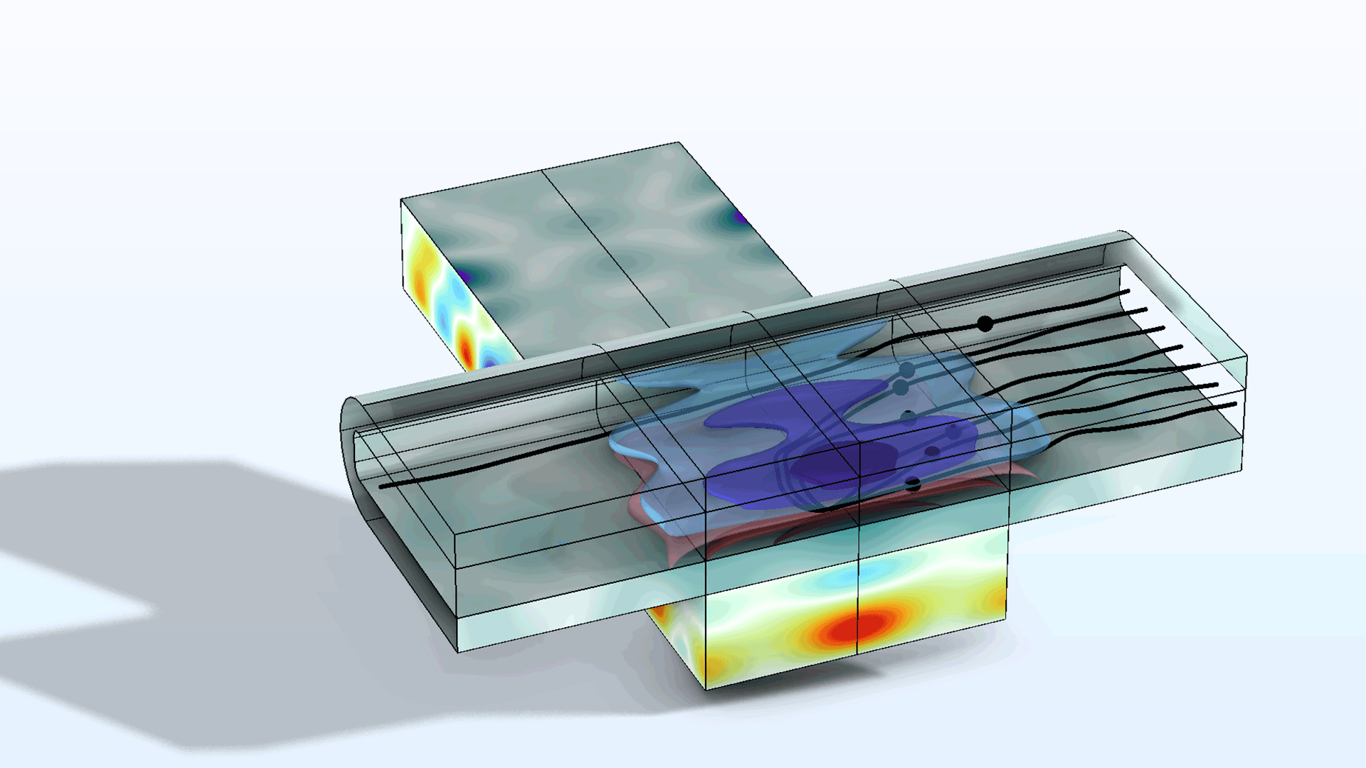
Thermoviscous Boundary Layer Impedance for the Acoustic–Structure Boundary Multiphysics Coupling

When coupling a vibrating structure to an acoustic domain using the Acoustic–Structure Boundary multiphysics coupling, a Thermoviscous Boundary Layer Impedance subfeature can now be added to the multiphysics coupling. This simplifies the setup of large vibroacoustics models where thermoviscous losses are included with the homogenized boundary condition formulation of the thermoviscous boundary layer impedance. This functionality is also important for speeding up certain shape optimization problems, or for faster approximate simulations. View this new addition in the Piezoelectric MEMS Speaker tutorial model.

The new Thermoviscous Boundary Layer Impedance feature for the Acoustic–Structure Boundary multiphysics coupling.

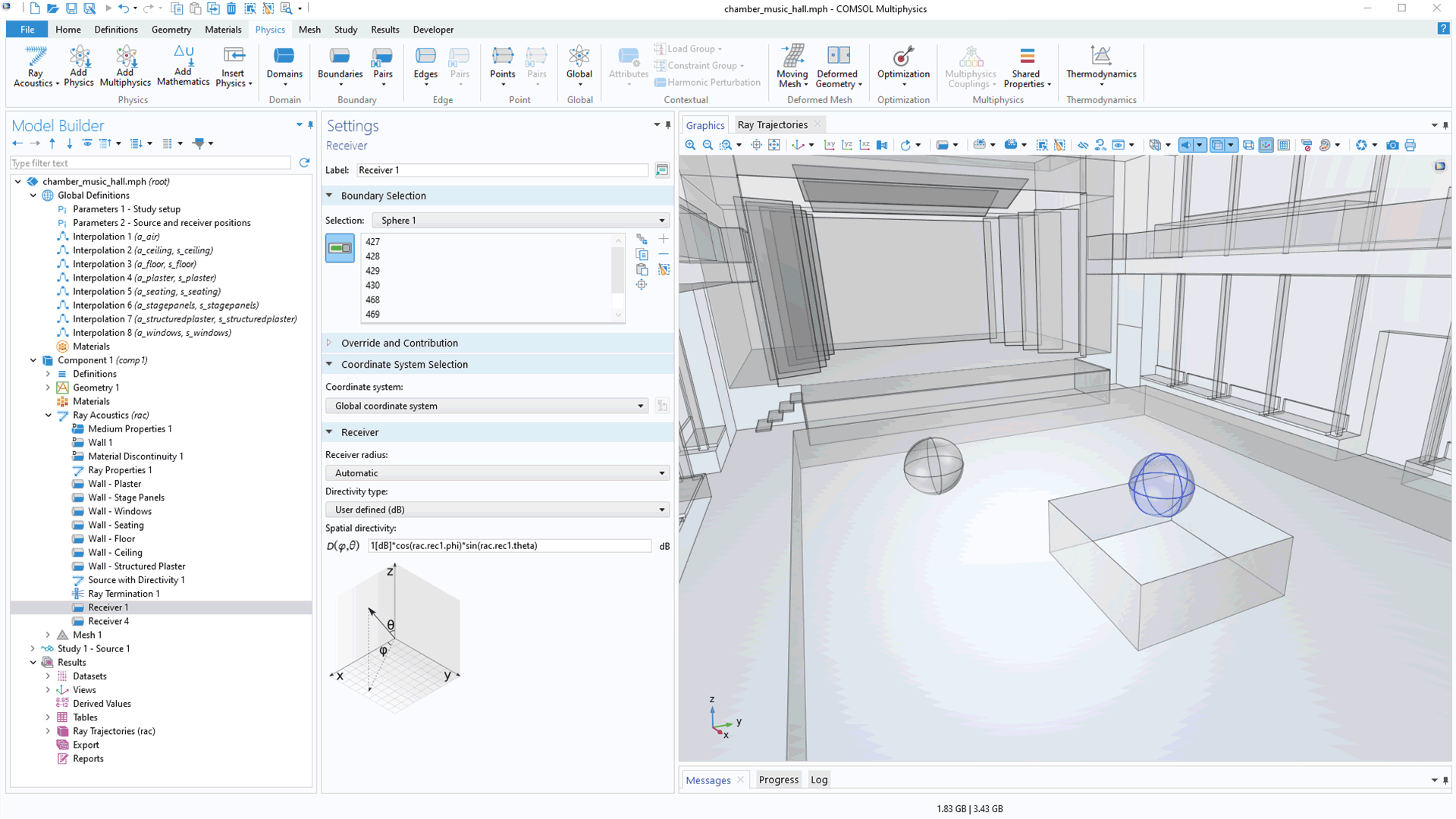
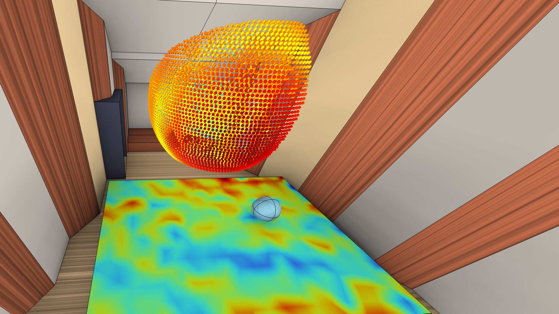
New Receiver Feature in Ray Acoustics

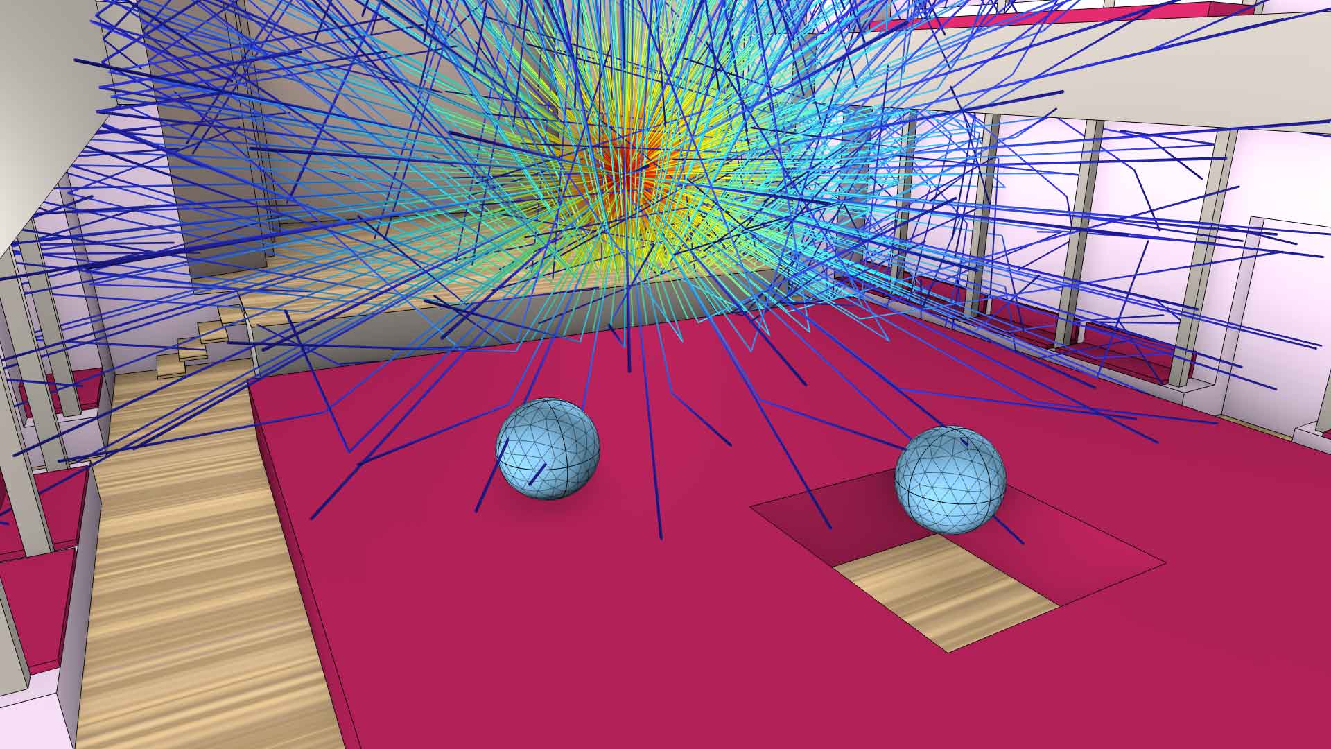
A new physics-based Receiver feature in the Ray Acoustics interface drastically improves performance for analyzing an impulse response. This feature is used to define the boundaries of a receiver sphere in the geometry when setting up the physics. The receiver collects information (arrival time and power) about the intersecting rays during the simulation. This information is then used for computing the impulse response in the results analysis. The combined computation and results analysis time (to compute impulse responses, plot ray trajectories, and more) for the Chamber Music Hall model has gone from 18 hours (when using version 6.1) to 2 hours (with version 6.2). The time to analyze the 10 impulse responses has decreased from 16 hours to 30 minutes (for 2 sources and 5 receivers, 10 pairs in all, using 46,000 rays, and using 18 bands with a 1/3 octave resolution). The Receiver feature is also showcased in the updated Small Concert Hall Acoustics tutorial model.

The Receiver feature settings for the Chamber Music Hall tutorial model.

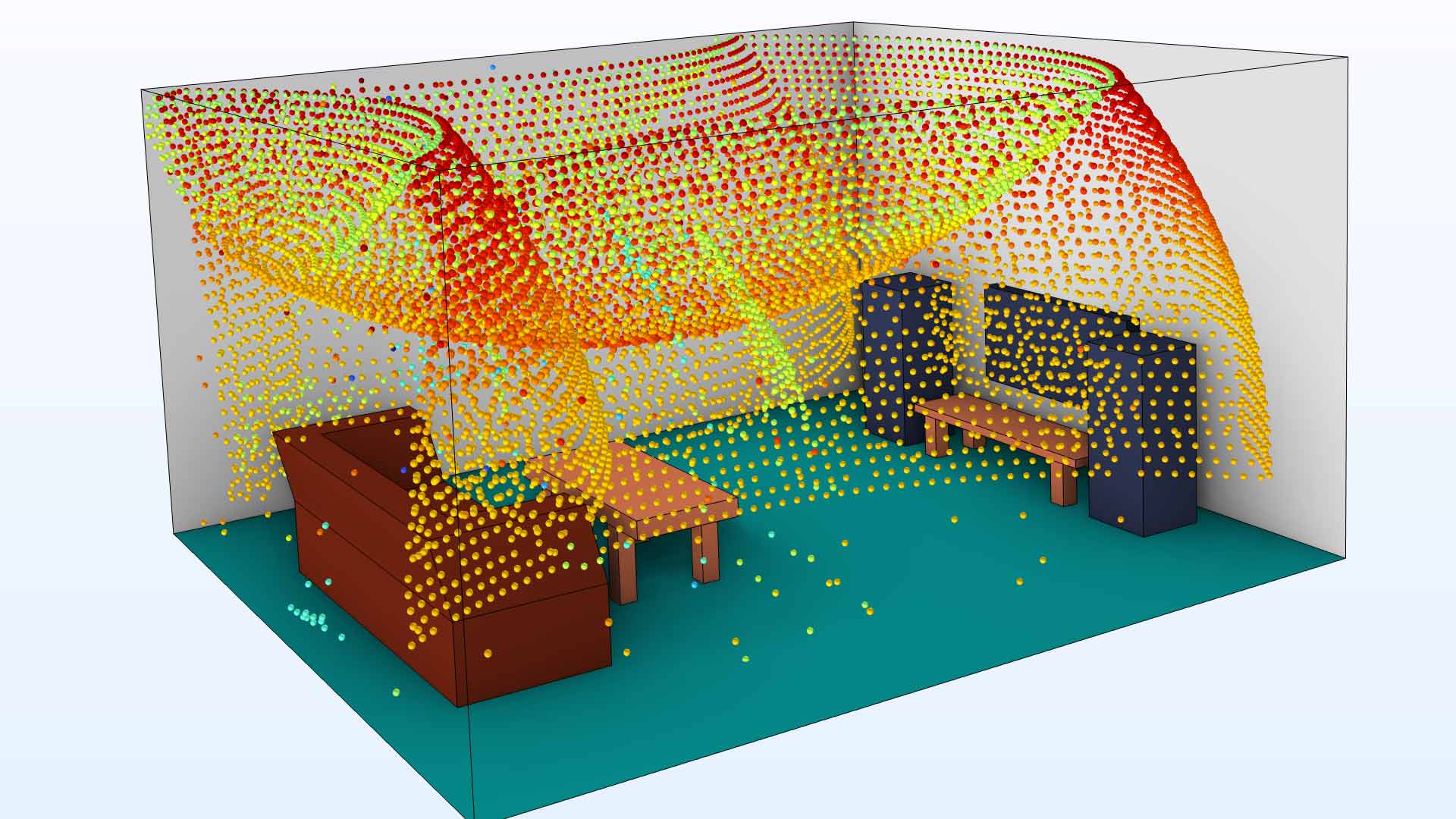
New Release from Pressure Field in Ray Acoustics

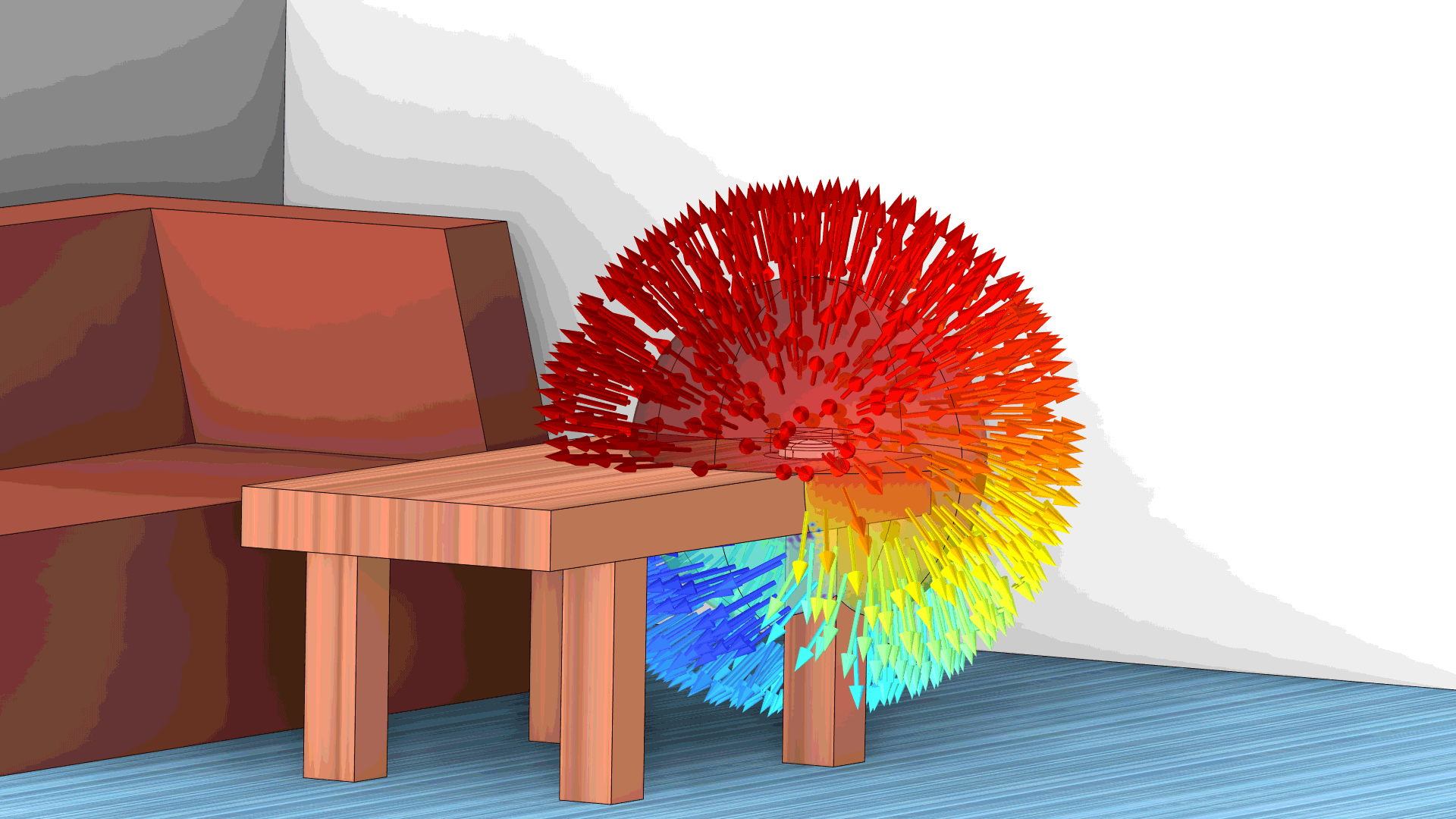
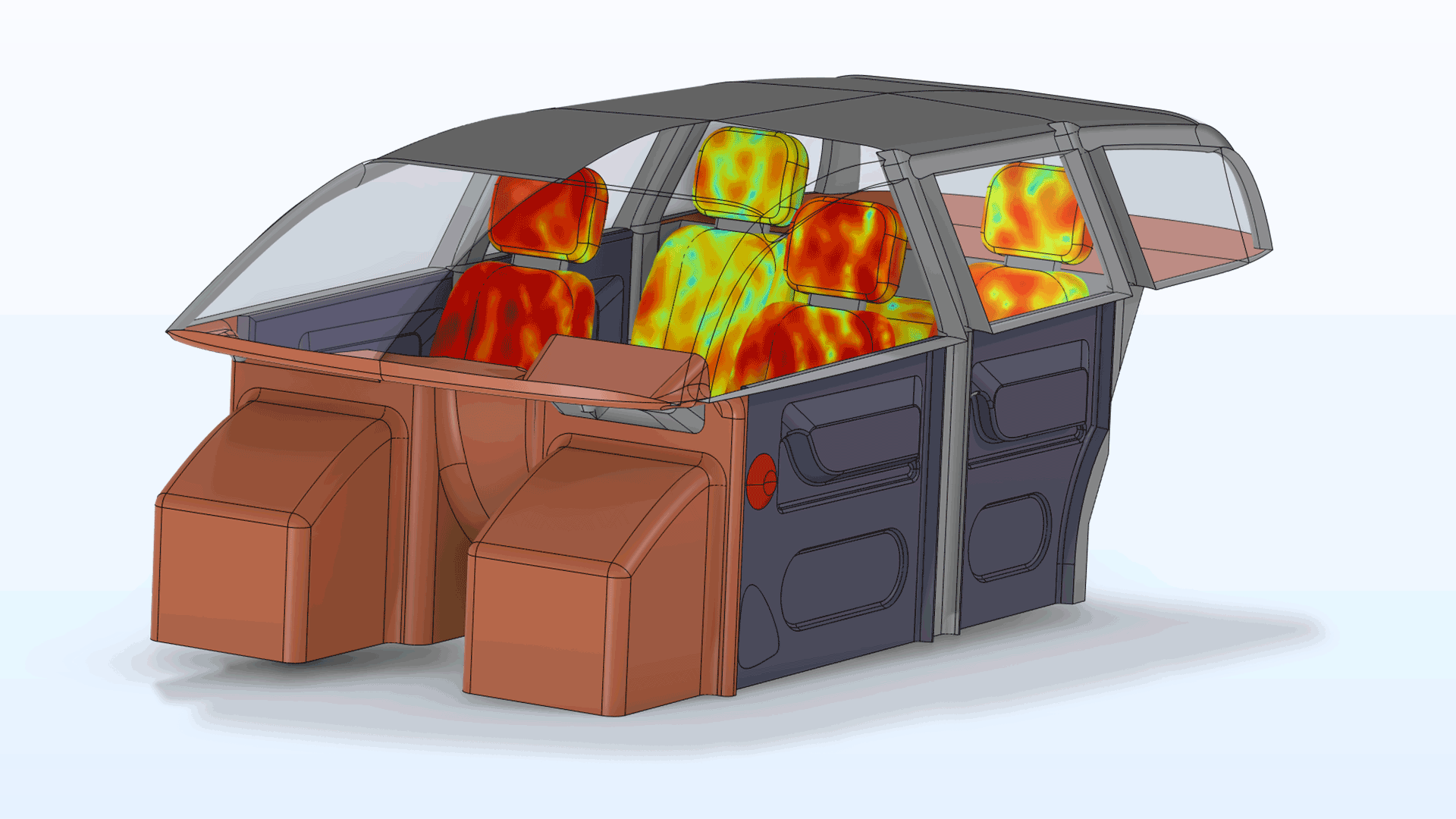
The new Release from Pressure Field feature is used to create realistic sources in the Ray Acoustics interface. The realistic source information is first extracted from a wave-based (near-field) simulation using the Pressure Acoustics, Frequency Domain interface. This means that the classical point source approximation of ray tracing is not always necessary. An example of a near-field source could be a loudspeaker placed in the dashboard of a car, where the placement causes local reflections and diffraction, as shown in the new Car Cabin Acoustics: Hybrid FEM–Ray Source Coupling tutorial model. In this case, ray tracing cannot capture the wave phenomena. However, by using a local pressure acoustics model, these phenomena can be addressed. The Release from Pressure Field feature enables the release of rays, where their magnitude and direction are determined by the intensity field within the pressure acoustics model. You can see this new feature in the Room Impulse Response of a Smart Speaker tutorial model.

The new Release from Pressure Field feature releases rays from a surface, with the magnitude and direction given by the intensity vector of the solved pressure acoustics model.

Import of WAV Audio Files

WAV audio files (.wav) can now be imported as Interpolation functions. This is useful for many applications in acoustics, such as when comparing simulations with measured data or when importing source signals for a transient analysis. You can see this new functionality in the updated Small Concert Hall Acoustics tutorial model.

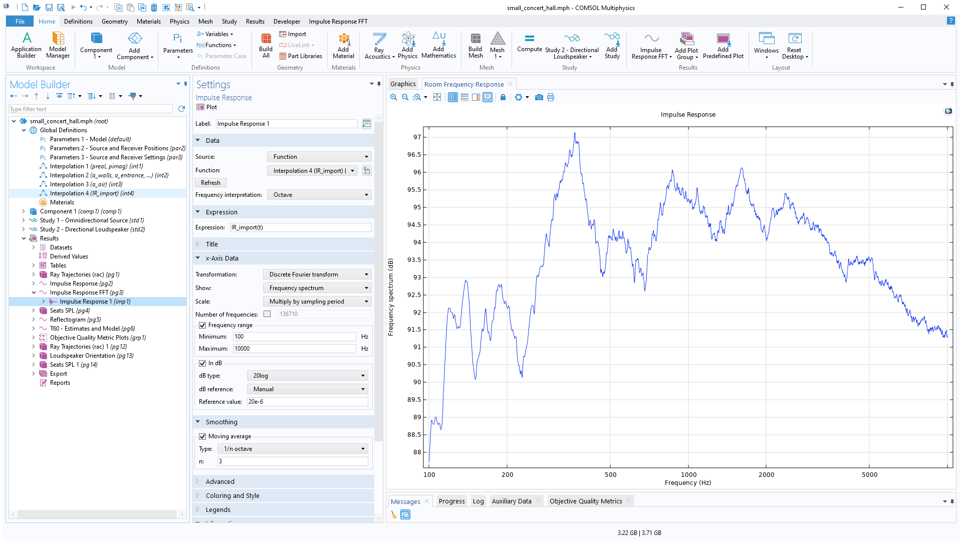
Functions as Source for the Impulse Response Plot

For the data source for the Impulse Response plot, there is now a Function option (as opposed to only a receiver dataset). This means that the Impulse Response plot can be used to analyze user-defined impulse response data, for example, based on a WAV audio file import. This functionality enables the analysis of measurement data as well as data resulting from a concatenation of low-frequency wave-based and high-frequency ray simulations. The Small Concert Hall Acoustics tutorial model showcases this new addition.

The new Source option in the Impulse Response plot allows for the analysis of imported signals or signals that are not taken from a ray acoustics simulation.

Updates to the Octave Band Plot

The Octave Band plot can now be used to analyze results based on a transient simulation. The transient data is transformed to the frequency domain before being analyzed. The Octave Band plot now also has a General (non-dB) input type that can be used to analyze absorption data in acoustics or vibration velocity data to plot a frequency response function (FRF) in a structural vibrations model.

Gradient-Based Optimization with Exterior Field Operator in 2D Axisymmetric Models

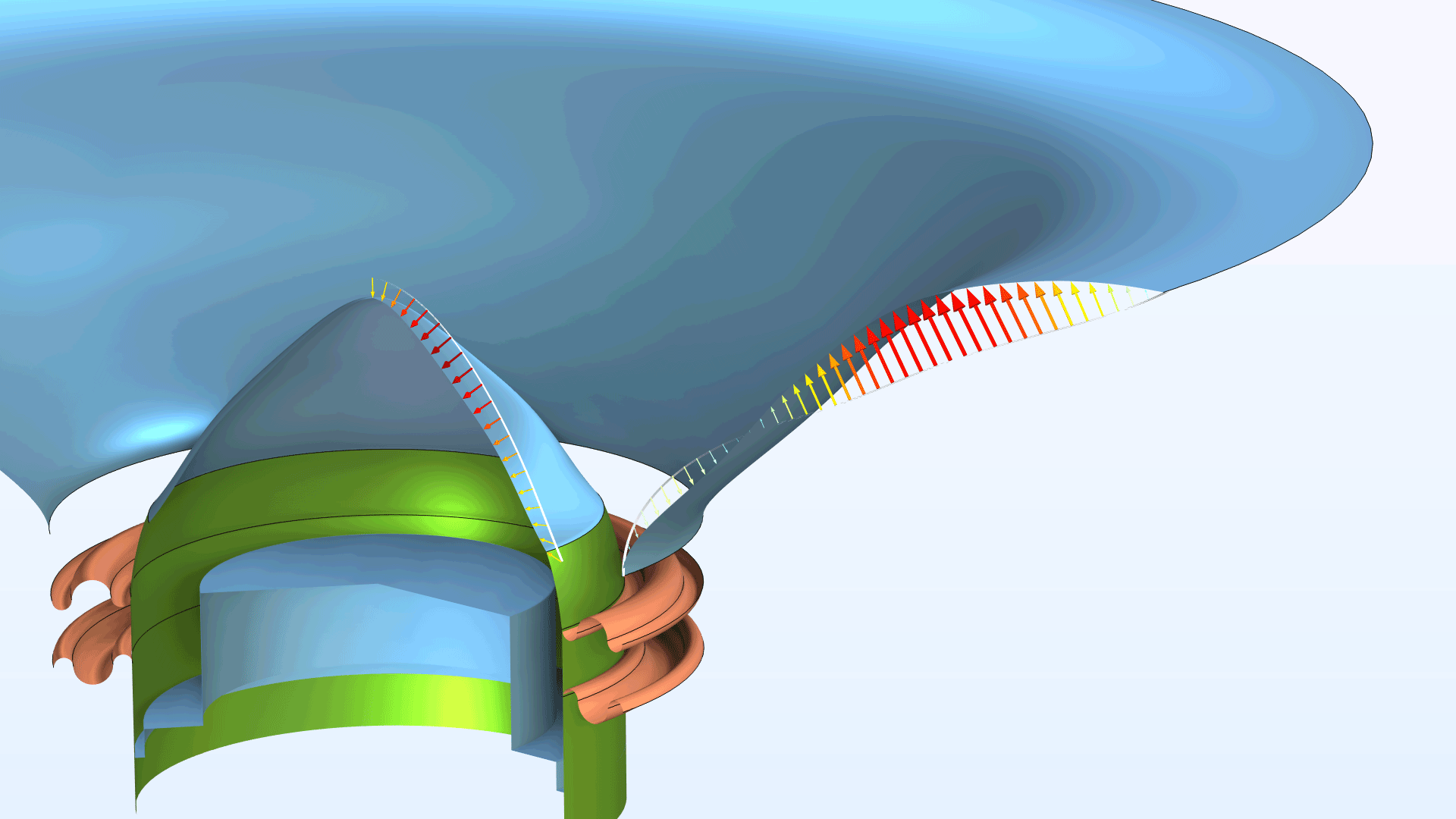
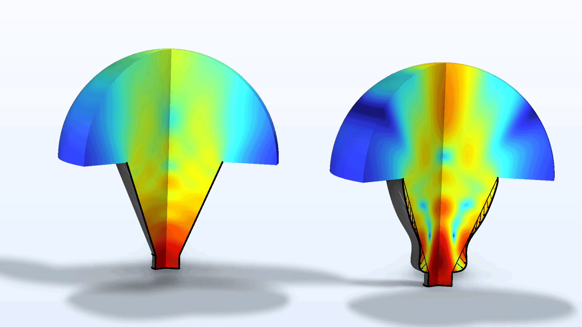
Gradient-based optimization (shape or topology optimization) is now supported in 2D axisymmetric models when using the dedicated optimization exterior-field Lp_pext_opt operator in the Pressure Acoustics, Frequency Domain interface. The optimization version of the exterior field operator, similar to the already existing operator in 3D, is implemented such that its sensitivity can be computed analytically. As an example, the Tweeter Dome and Waveguide Shape Optimization tutorial model has been updated to use the new operator; consequently, the acoustic domain can now be greatly reduced, and the model runs 50% faster. You can also see this update in the Optimizing the Shape of a Horn tutorial model.

Shape optimization of a tweeter dome and waveguide using the new Lp_pext_opt operator.

First-Order Material Contributions in Acoustic Streaming

A new option to include the first-order material dependency of viscosity has been added to the multiphysics couplings for acoustic streaming. This effect is typically important in a rotating streaming flow generated by a combination of two resonances, generating a rotating acoustic wave.

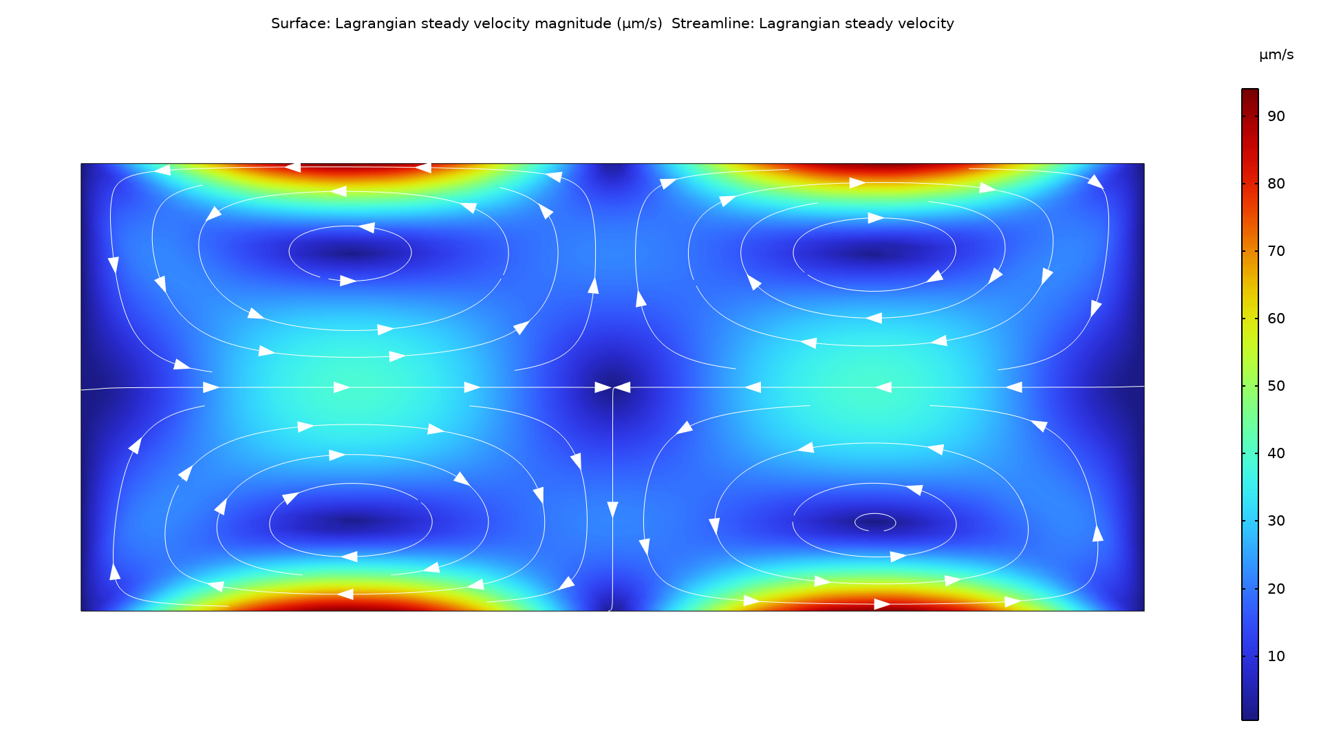
Lagrangian Steady Velocity Variables in Acoustic Streaming

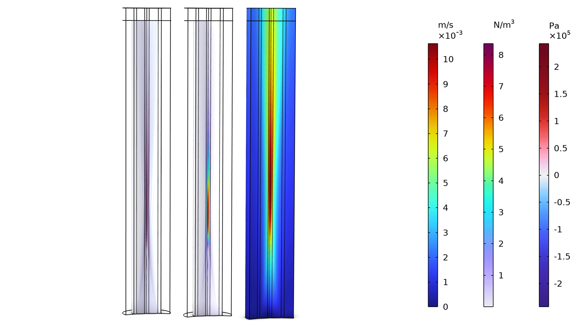
New predefined variables have been added for the Lagrangian steady velocity when modeling acoustic streaming. This velocity should be used when computing the trajectories of particles in a streaming flow. The variable is announced in the user interface and can easily be selected as input for the viscous drag force in, for example, the Particle Tracing for Fluid Flow physics interface. You can view this in the Acoustic Streaming in a Microchannel Cross Section tutorial model.

The Lagrangian streaming velocity in a microchannel cross section, based on predefined variables.

New Adaptive Frequency Sweep Study

A new frequency-domain study type called Adaptive Frequency Sweep has been added to the Pressure Acoustics, Frequency Domain interface. The study is useful for performing dense frequency sweeps in an efficient manner using the asymptotic waveform evaluation (AWE) method. The study requires the input of a metric that keeps track of the acoustic response of the modeled system. View this new study type in the Helmholtz Resonator Analyzed with Different Frequency Domain Solvers tutorial model.

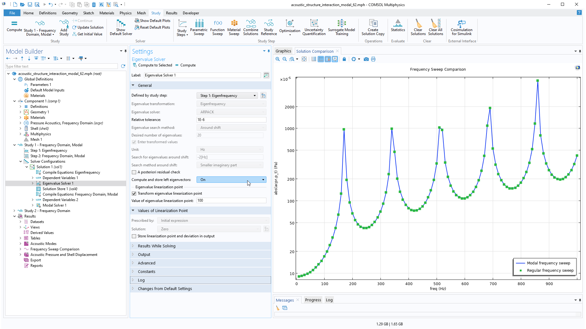
Frequency Modal for Vibroacoustics Models

You can now perform analyses of vibroacoustics multiphysics models using the modal solver. This is made possible since both the left and right eigenvectors are now computed when performing an eigenfrequency analysis. This functionality is shown in the Acoustic–Structure Interaction with Frequency Domain, Modal Solver tutorial model.

Use of the Frequency Domain, Modal solver for a vibroacoustics (acoustic–structure interaction) problem.

Performance Improvements for BEM Acoustics Models

Several important improvements have been introduced for solving acoustics models with the boundary element method (BEM) using the Pressure Acoustics, Boundary Elements interface.

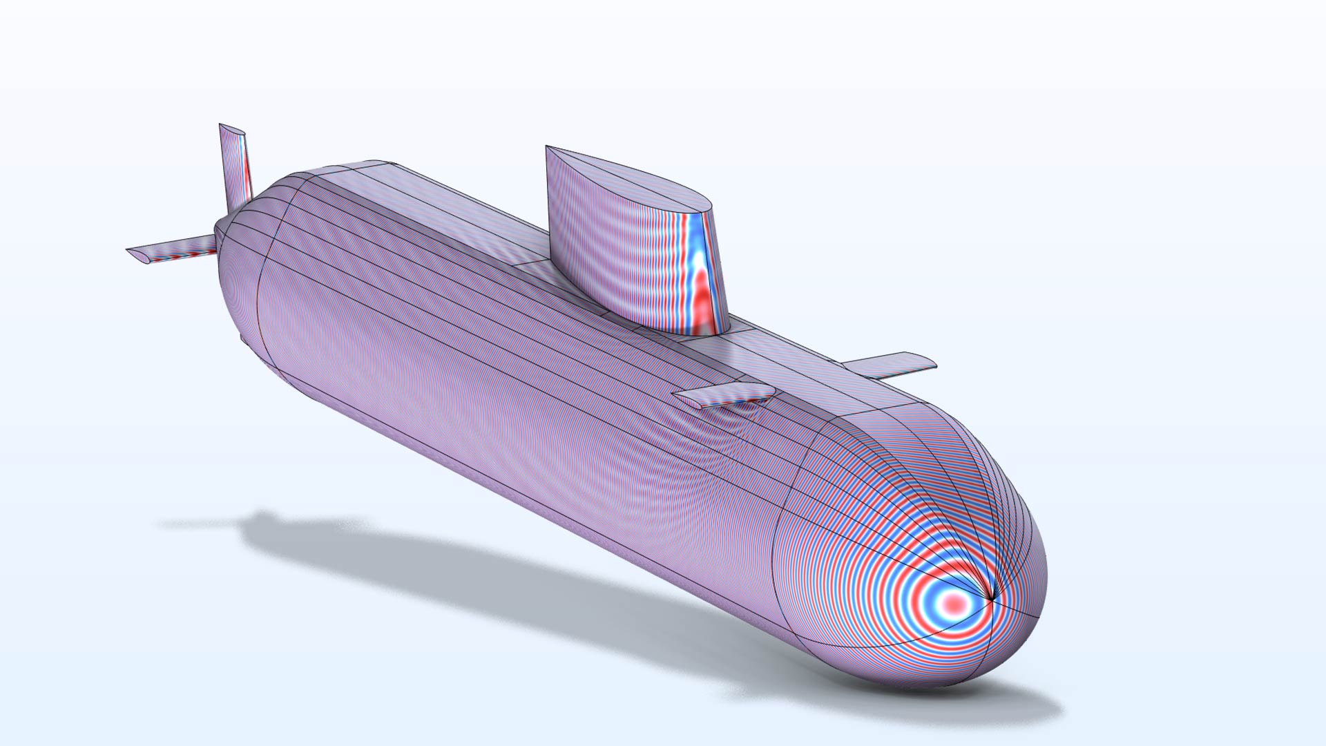
• The evaluation of the BEM kernel for complex-valued wave numbers (models with fluid attenuation) has been optimized. As an example, generating the Radiation Pattern plot in the Submarine Target Strength model is now 25% faster. The speedup depends on the model size and hardware.
• Load and memory balancing for BEM models run on clusters has been greatly improved. As an example, solving the Submarine Target Strength model at 6 kHz on 6 nodes on a cluster is now 7.5 times faster in version 6.2 than in the previous version — the model now solves in 55 minutes instead of 7 hours 30 minutes. The peak memory and memory balancing have also been greatly improved, enabling substantial speedup for solving large acoustics problems. The speedup is problem and hardware dependent.
• An improved solver is now also available for solving models that use the stabilized BEM method in noncluster configurations (on a regular workstation). As an example, the Submarine Target Strength model now solves in 16 minutes, compared to the 25 minutes it takes in version 6.1 (solved at 1.5 kHz). The speedup is problem and hardware dependent. Classical (nonstabilized) BEM problems also show a small speedup.
• There is a new quadrature option that can be enabled to improve thin-gap handling. This is relevant for sound radiation through thin waveguides, if solved with BEM.

The Submarine Target Strength tutorial model solved at 6 kHz. The image shows the total pressure at the submarine surface. This is a BEM model with 2.5 million degrees of freedom, and the submarine length corresponds to 250 wavelengths.

Additional Enhancements and Improvements

• Improved handling of the symmetry axis when modeling in 2D axisymmetry with the interfaces for thermoviscous acoustics, linearized Navier–Stokes equations, and linearized Euler equations, in particular, taking the azimuthal mode number into account (for m = 0, m = 1, and m > 1)
• Handling of symmetry on a circular port in the Thermoviscous Acoustics, Frequency Domain interface without warning
• Intensity variables for the total, background, and scattered fields in the interfaces for thermoviscous acoustics and linearized Navier–Stokes equations
• No correction option for the back volume added to the Lumped Speaker Boundary condition in thermoviscous acoustics and pressure acoustics
• Option to automatically pick up solid velocities as sources in the Pressure Acoustics, Kirchhoff–Helmholtz interface
• Ports in elastic wave problems solved with the Solid Mechanics interface now correctly handle nonorthogonal higher-order modes
• Out-of-plane contributions now included in the source terms in the interfaces for thermoviscous acoustics, linearized Navier–Stokes equations, and linearized Euler equations

New and Updated Tutorial Models

COMSOL Multiphysics^® version 6.2 brings several new and updated tutorial models to the Acoustics Module.

Wave-Based Time-Domain Room Acoustics with Frequency-Dependent Impedance

A wave-based analysis of the acoustics of a room, including frequency-dependent impedance conditions in the time domain. Wall impedance data analyzed via the Partial Fraction Fit function and the new Impedance boundary condition in the time domain.

Application Library Title:
full_wave_transient_room_acoustics
Download from the Application Gallery

MEMS Microphone with Slip Wall

A MEMS microphone solved in the frequency domain, including the DC prestress effects. The model uses the new Slip Wall boundary condition to include the effects of high Knudsen numbers, which are important for the acoustic response of the microperforated plate (MPP) and for the squeezing flow.

Application Library Title:
mems_microphone_slip_wall
Download from the Application Gallery

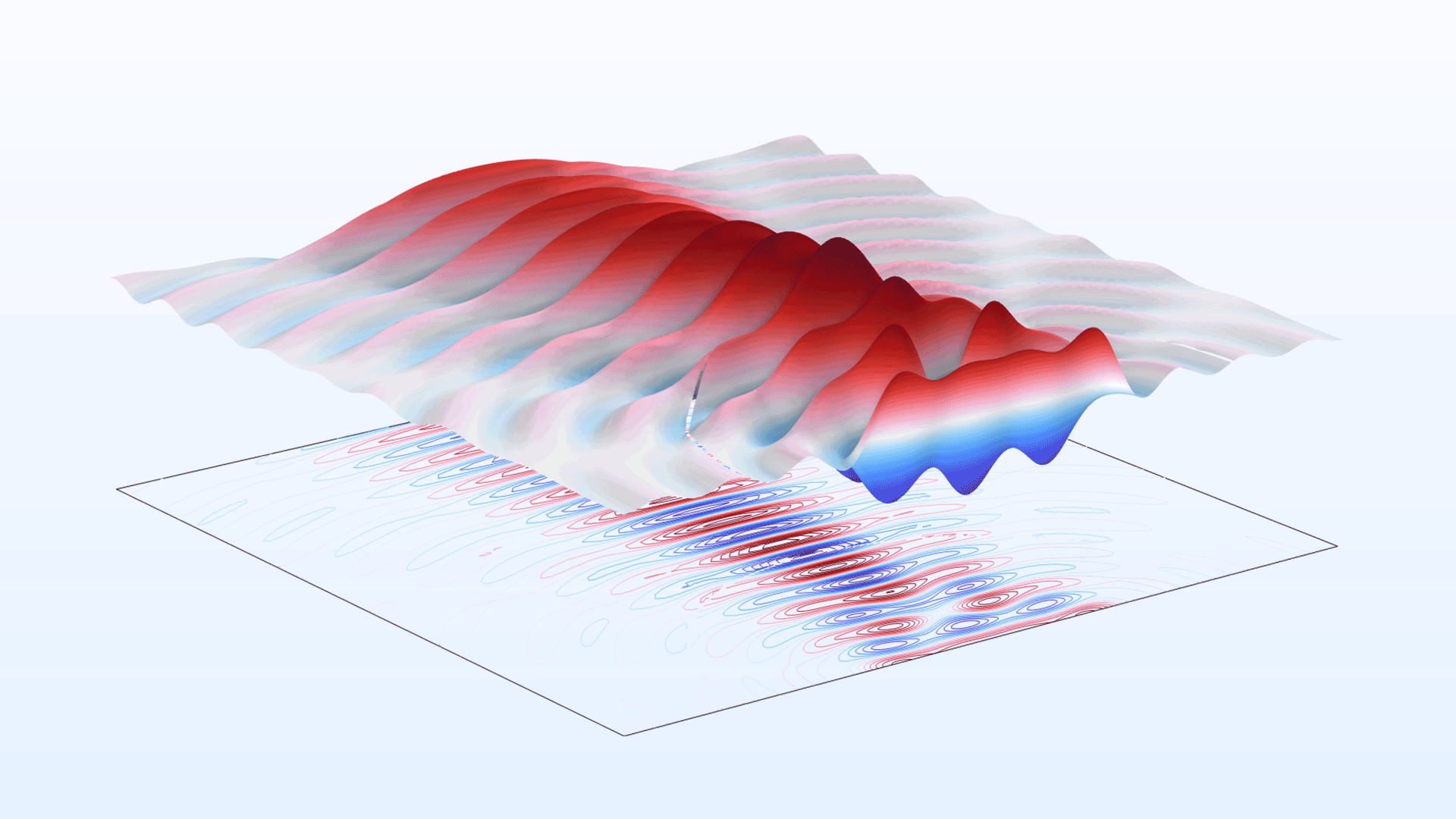
Generation of Lamb Waves for Nondestructive Inspection of Plate Specimens

An analysis of a nondestructive testing (NDT) setup for the inspection of a steel plate with a finite width and thickness. An angle beam wedge excites the desired surface mode in the plate, which is used to detect a defect.

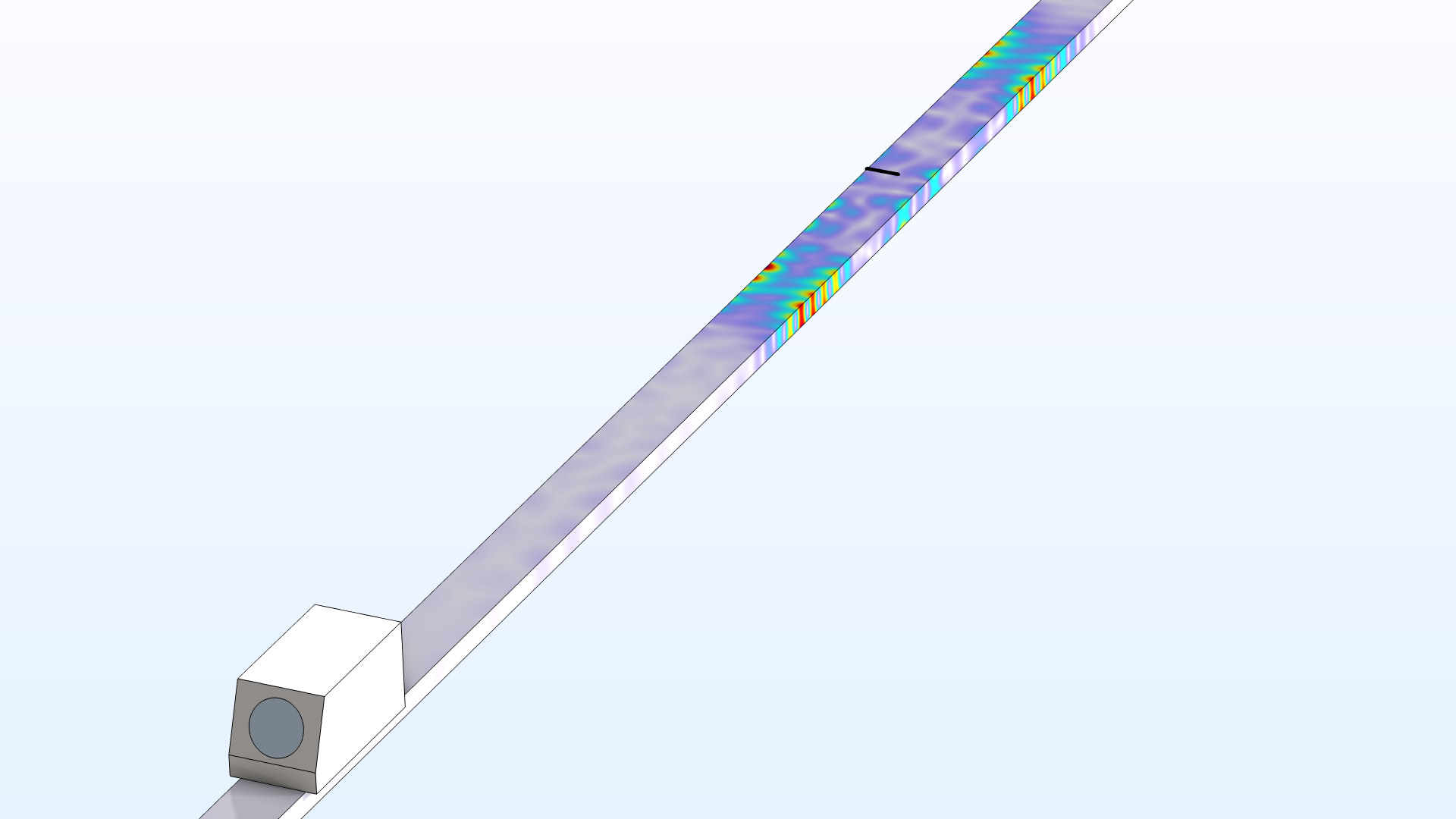
Application Library Title:
lamb_waves_ndt_plate
Download from the Application Gallery

Viscous Damping of a Microperforated Plate in the Slip Flow Regime

An acoustic analysis of the input impedance of an MPP model. The model shows the importance of the Slip Wall boundary condition and finds the optimal hole size for the MPP.

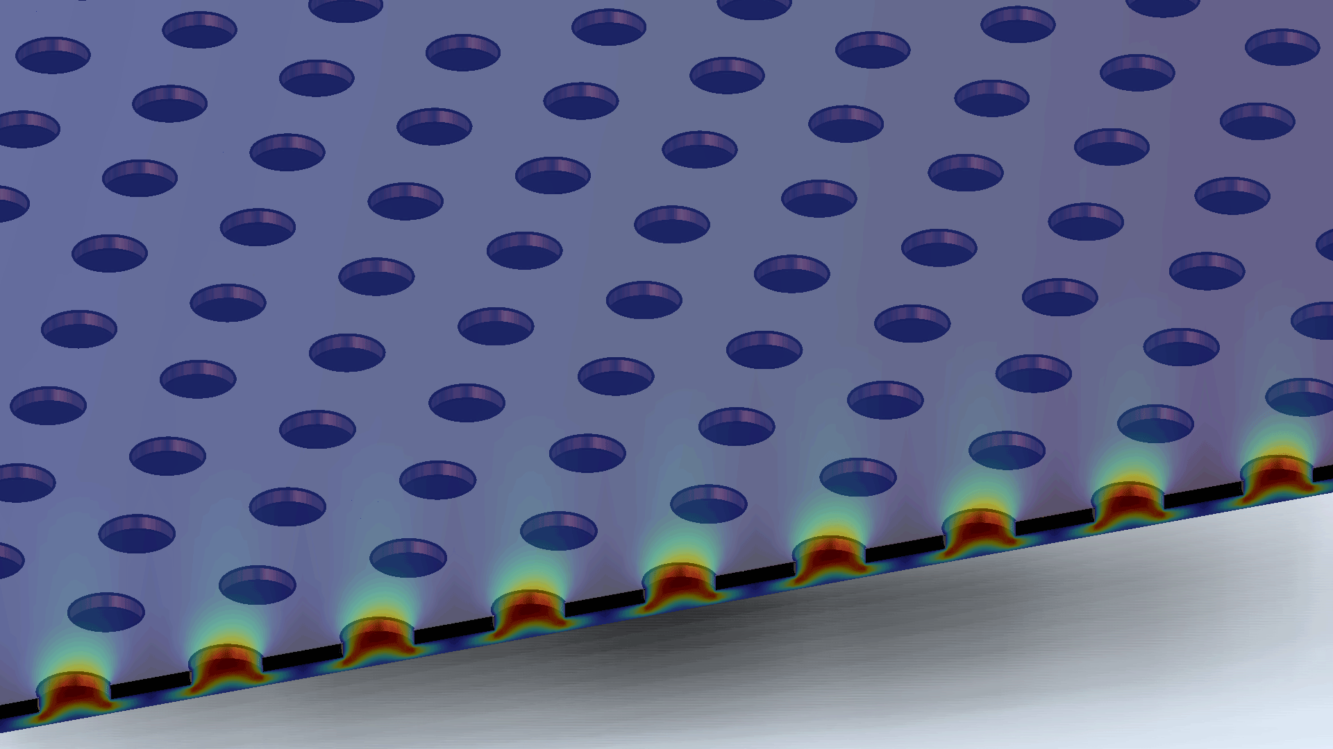
Application Library Title:
viscous_damping_mpp
Download from the Application Gallery

Car Cabin Acoustics — Frequency-Domain Analysis

This model analyzes the low-frequency to midfrequency range performance of the sound system in a car cabin. The frequency response at the location of a microphone array and the modal behavior at low frequencies are computed.

Application Library Title:
car_cabin_acoustics
Download from the Application Gallery

Baffled Piston Radiation

The validation model of the classical baffled piston radiation problem, comparing the simulation results to the analytical solution.

Application Library Title:
baffled_piston_radiation
Download from the Application Gallery

Loudspeaker Driver 3D — Frequency-Domain Analysis

A full frequency-domain analysis of a 3D vibroelectroacoustic multiphysics model of a loudspeaker.

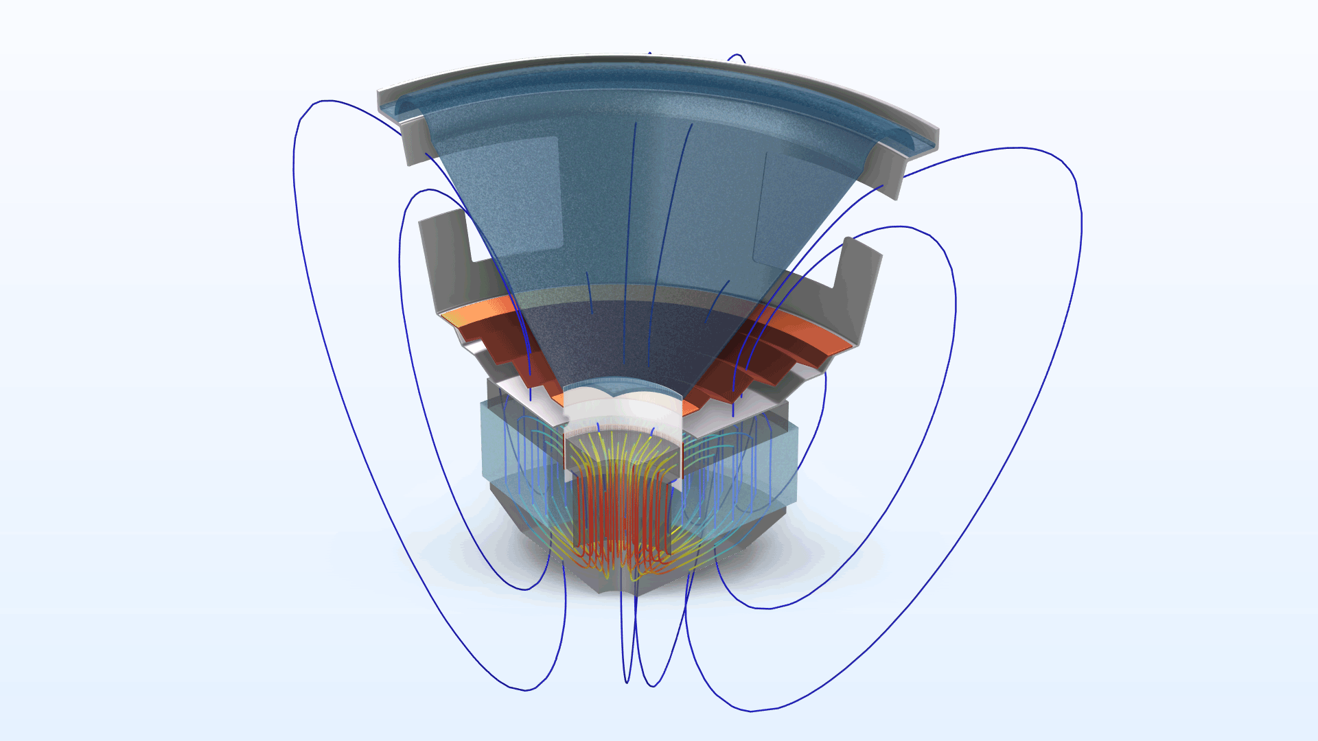
Application Library Title:
loudspeaker_driver_3d
Download from the Application Gallery

Eigenmodes in Air Bubble with Surface Tension

An analysis of the eigenmodes and eigenfrequencies of a micro air bubble in water is modeled and compared with analytical solutions.

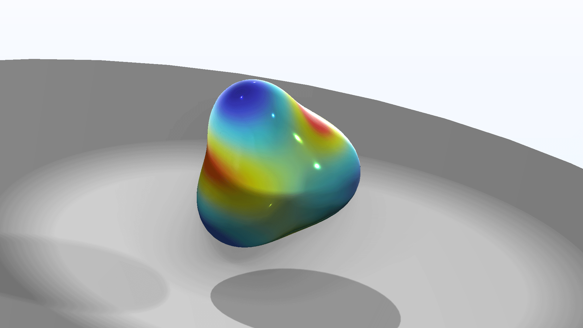
Application Library Title:
eigenmodes_air_bubble
Download from the Application Gallery

Scattered Field Formulation for Elastic Waves

P and S waves impinging on a cavity, a rigid inclusion, and an elastic inclusion.

Application Library Title:
scattered_field_elastic_waves
Download from the Application Gallery

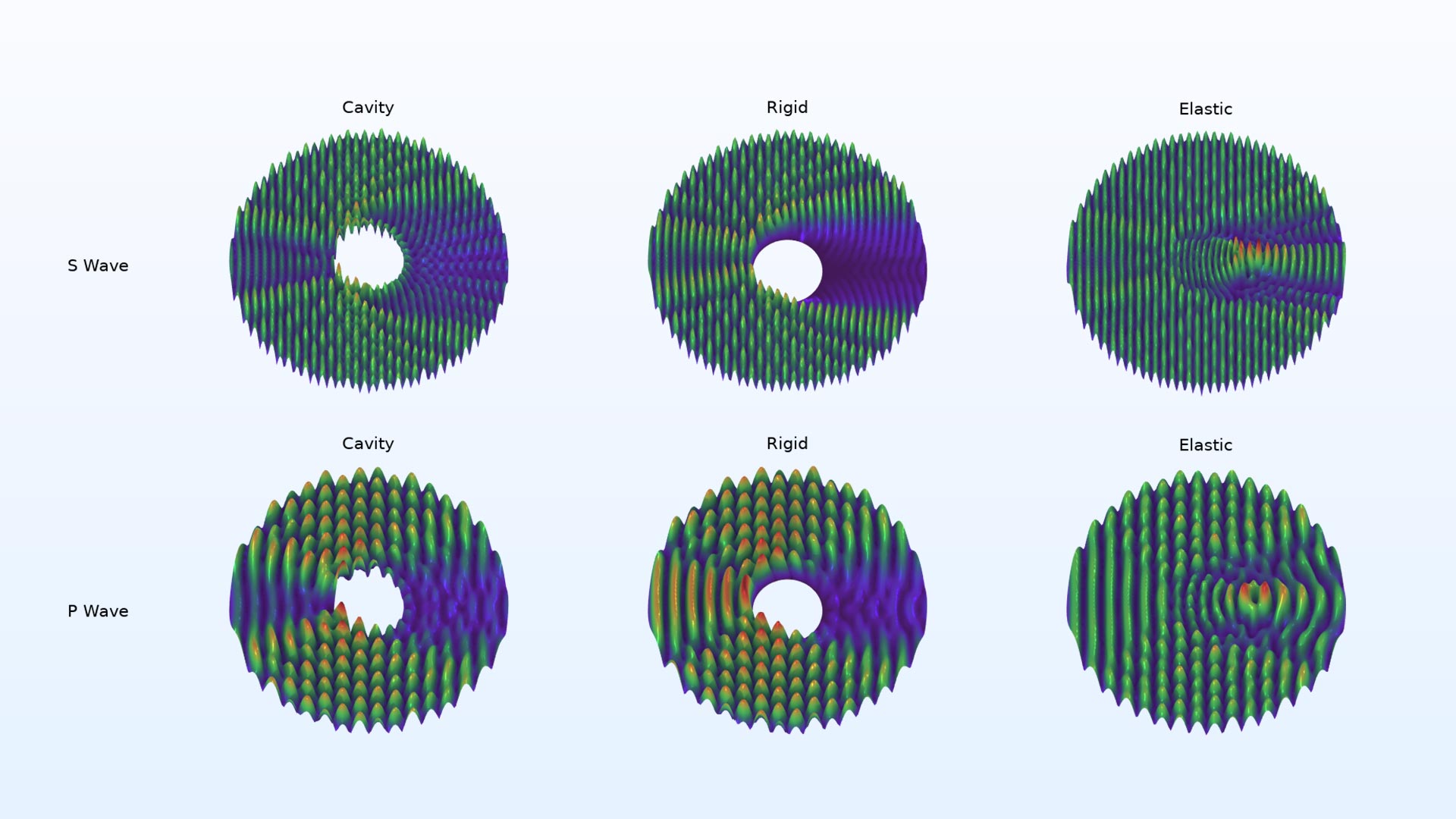
Elastic Cloaking with Polar Material

A comparison between the free field generated by a point load and the field around a cloaked obstacle.

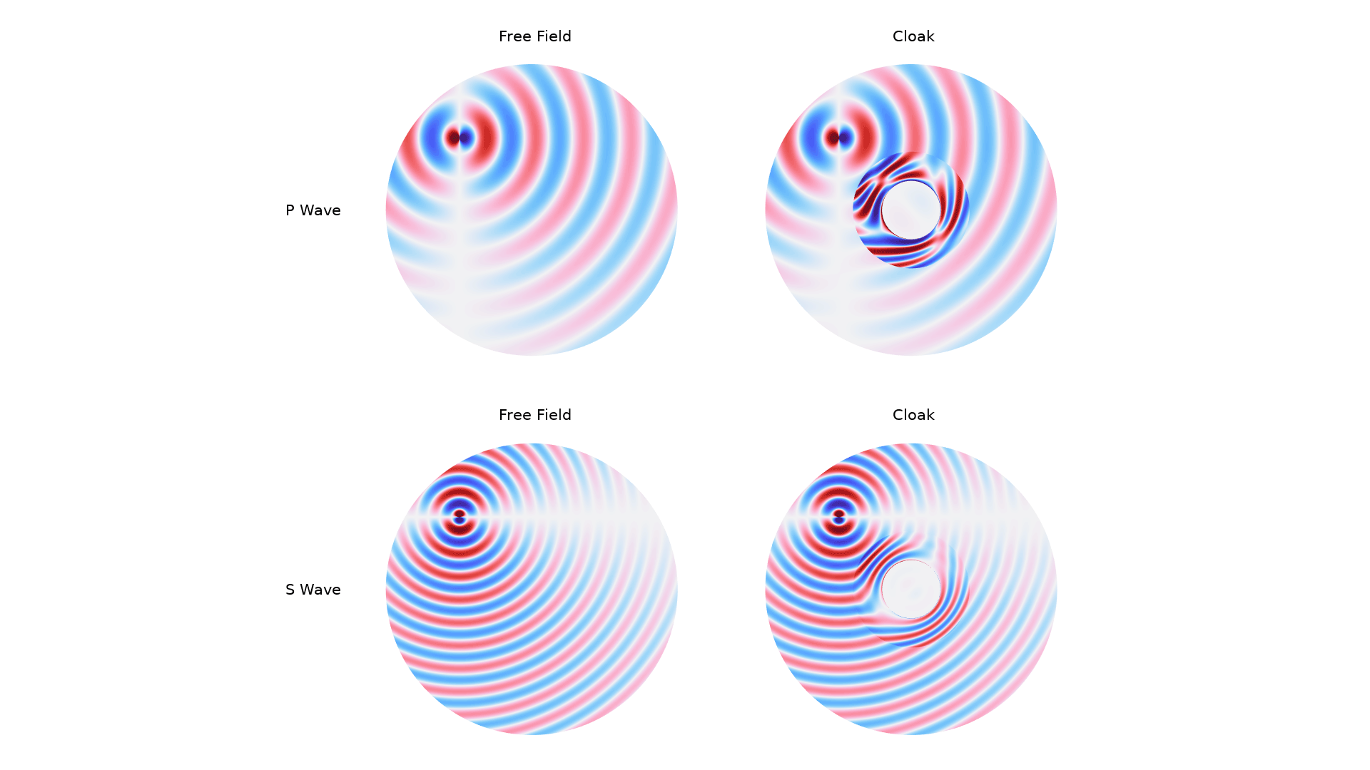
Application Library Title:
elastic_cloaking
Download from the Application Gallery

Thermoacoustic Engine and Heat Pump

Acoustic velocity and temperature fluctuations in the heat exchanger of a thermoacoustic heat engine and heat pump.

Application Library Title:
thermoacoustic_engine_heat_pump
Download from the Application Gallery

Fuel Tank Vibration

A full multiphysics analysis of the vibration behavior of a partially filled fuel tank. The model compares the results with the less accurate added-mass approach.

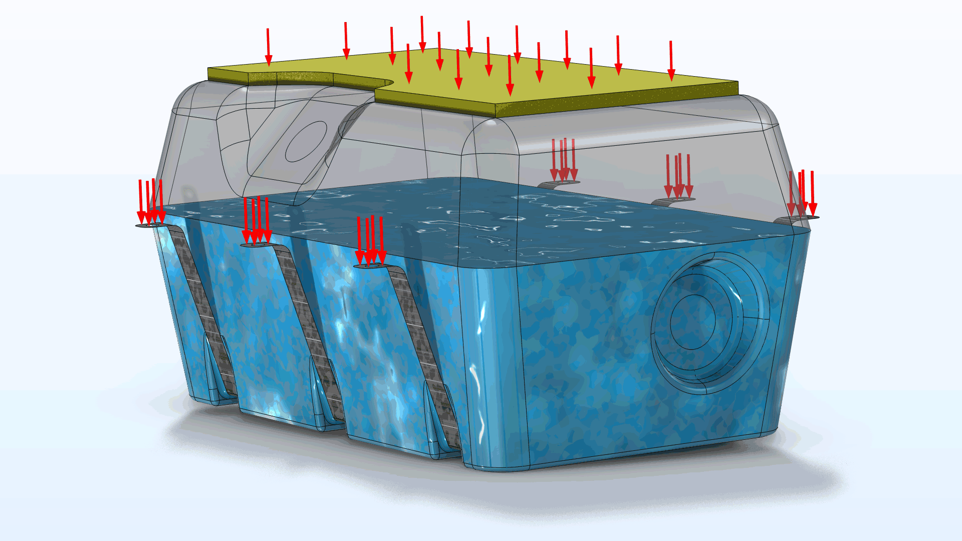
Application Library Title:
fuel_tank_vibration
Download from the Application Gallery

Nonlinear Transfer Impedance of a Tapered Orifice

Vortex shedding in a tapered orifice inducing local nonlinear acoustic losses. The transfer impedance of the system is analyzed and compared to results from the literature.

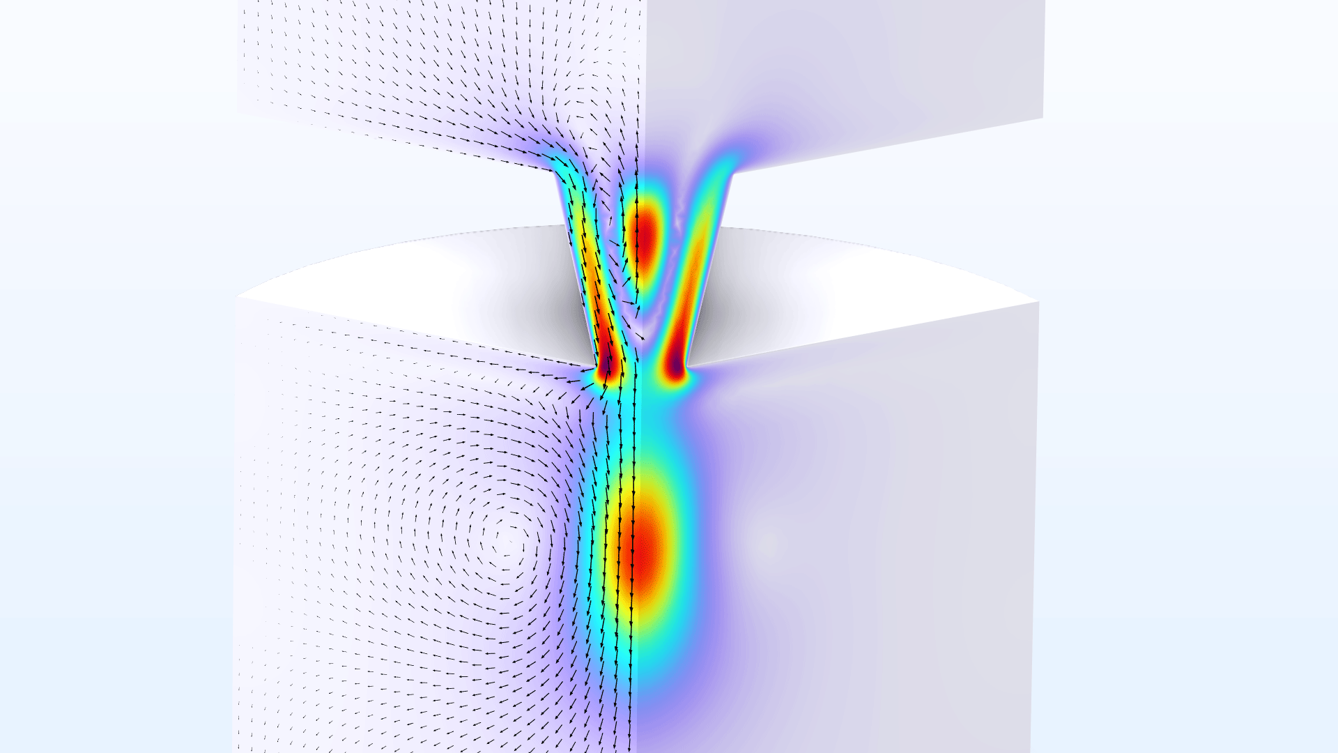
Application Library Title:
nonlinear_transfer_impedance
Download from the Application Gallery

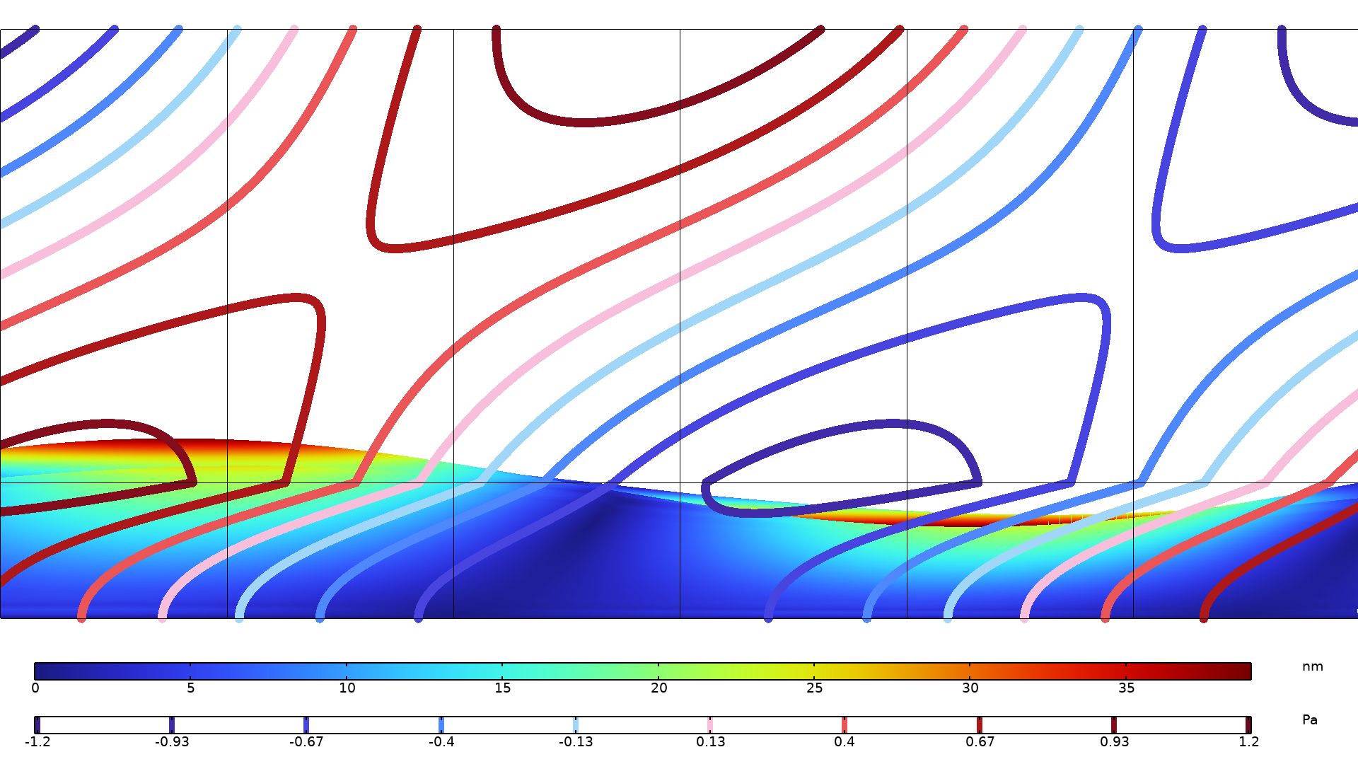
Type 4.3 Ear Simulator

This model is of the P.57 Type 4.3 Full-Band Ear Simulator. The model includes the geometry of the ear canal as well as the pinna defined in the ITU-T P.57 standard. The acoustic response of the system is analyzed and validated.

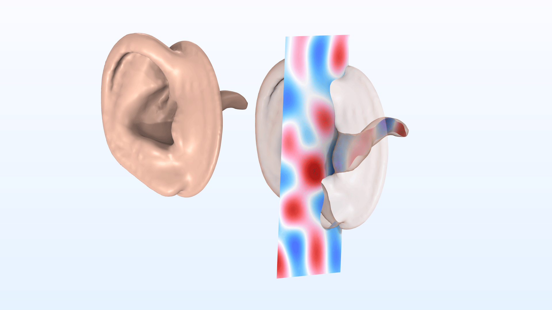
Application Library Title:
type_43_ear_simulator
Download from the Application Gallery

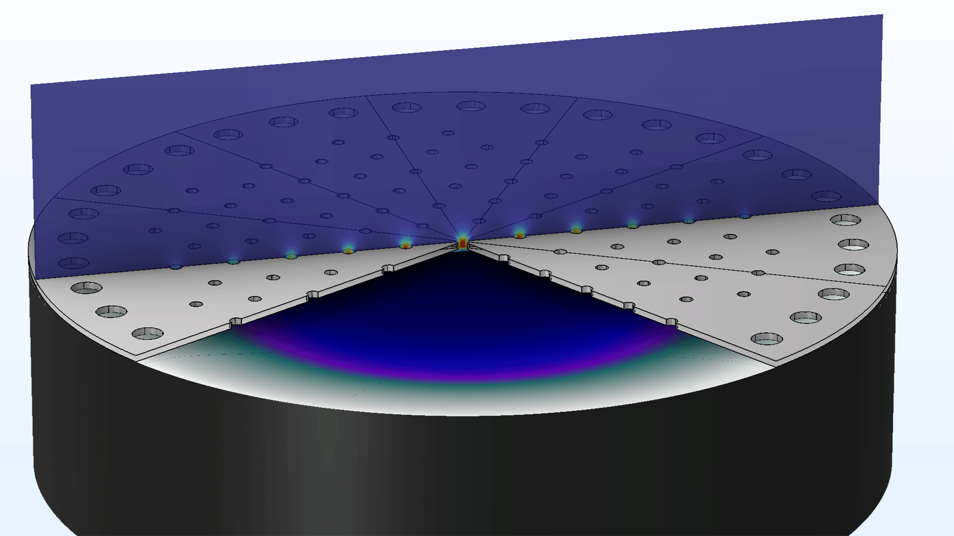
Transverse Isotropic Porous Layer

Investigating the acoustic properties of a porous layer made of glass wool. The porous material has transverse isotropic properties and is modeled with the full anisotropic poroelastic material model.

Application Library Title:
transverse_isotropic_porous_layer
Download from the Application Gallery

Active Flame Validation

The standing acoustic modes in the Active Flame Validation tutorial model, which demonstrates how to model the interaction between an acoustic field and the heat released from a flame using the new Flame Model feature.

Application Library Title:
active_flame_validation
Download from the Application Gallery

Small Concert Hall Acoustics

The Small Concert Hall tutorial model has been updated to include the new Receiver feature. The model also demonstrates the import of an audio WAV file.

Application Library Title:
small_concert_hall
Download from the Application Gallery

Chamber Music Hall

The Chamber Music Hall tutorial model has been updated to use the new Receiver feature for a more efficient impulse response analysis.

Application Library Title:
chamber_music_hall
Download from the Application Gallery

Flow Duct

The acoustic modal sound transmission analysis of a turbojet engine flow duct model, using the new Port boundary condition.

Application Library Title:
flow_duct
Download from the Application Gallery

Axisymmetric Condenser Microphone

The Axisymmetric Condenser Microphone model has been updated to use a more realistic geometry and has an additional capacitance study.

Application Library Title:
condenser_microphone
Download from the Application Gallery

Optimizing the Shape of a Horn

The shape optimization of a simple horn model. The model has been simplified because the Lppextopt operator now supports axisymmetric models.

Application Library Title:
horn_shape_optimization
Download from the Application Gallery

Tweeter Dome and Waveguide Shape Optimization

Shape optimization is used to obtain a uniform response for an acoustic tweeter with respect to frequency as well as angle. This model has been simplified because the Lppextopt operator now supports axisymmetric models.

Application Library Title:
tweeter_shape_optimization
Download from the Application Gallery

Acoustic Streaming Induced by a Focused Ultrasound Beam

Acoustic streaming, a steady flow induced by sound waves, is used in industrial biomedical and engineering applications. Examples include the enhancement of convective heat transfer, ultrasonic cleaning, localized micromixing, hemolysis of blood cells, micropumps, etc.

Download from the Application Gallery

Opto-Acoustophoretic Effect in an Acoustofluidic Trap

Opto-acoustophoresis is a term used to describe the interplay between acoustics and optical fields. In most cases (including in this model), the optical field heats up the material and therefore affects the acoustic field.

Download from the Application Gallery

Acoustic Trap in Glass Capillary with Bias Flow

A 3D model of an acoustic trap in a glass capillary with a bias flow. The model includes the drag forces from an acoustic streaming flow and bias flow, as well as radiation forces on small particles.

Download from the Application Gallery

Room Impulse Response of a Smart Speaker

This model combines pressure acoustics and ray acoustics to perform a full frequency-range analysis of the room impulse response of a small smart speaker. The source characterization in the ray-tracing model is based on a full multiphysics model of the transducer and uses the Release from Pressure Field feature to set up the transducer source.

Download from the Application Gallery

Smartphone Microspeaker and Port Acoustics: Linear and Nonlinear Analysis

Analysis of a microspeaker located in a smartphone, including the radiation through, and interaction with, the acoustic port that connects to the exterior. The model demonstrates a linear frequency-domain analysis as well as a nonlinear time-domain analysis.

Download from the Application Gallery

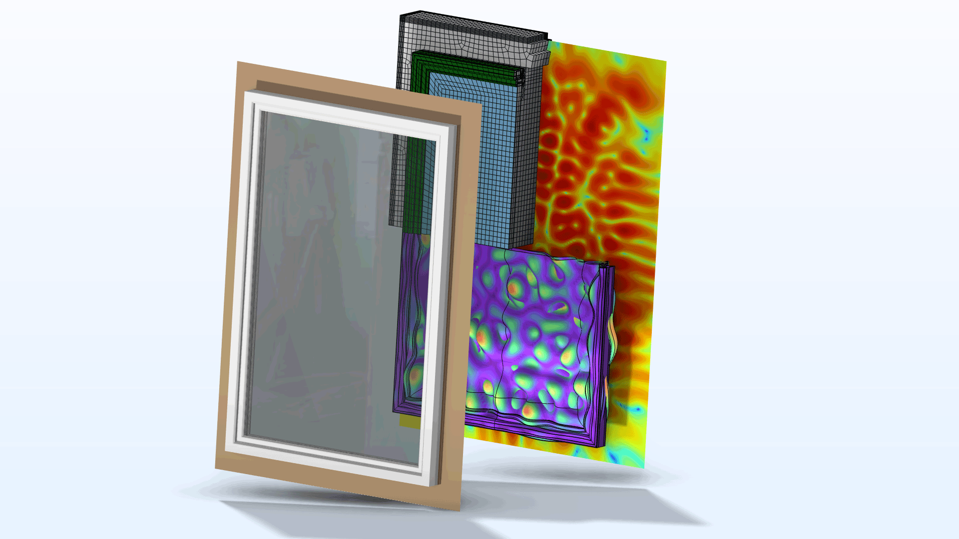
Sound Transmission Loss Through a Window

This model presents a practical and efficient method for computing the sound transmission loss (STL) through a building component. Specifically, this example treats the case of a double-glazed window.

Download from the Application Gallery

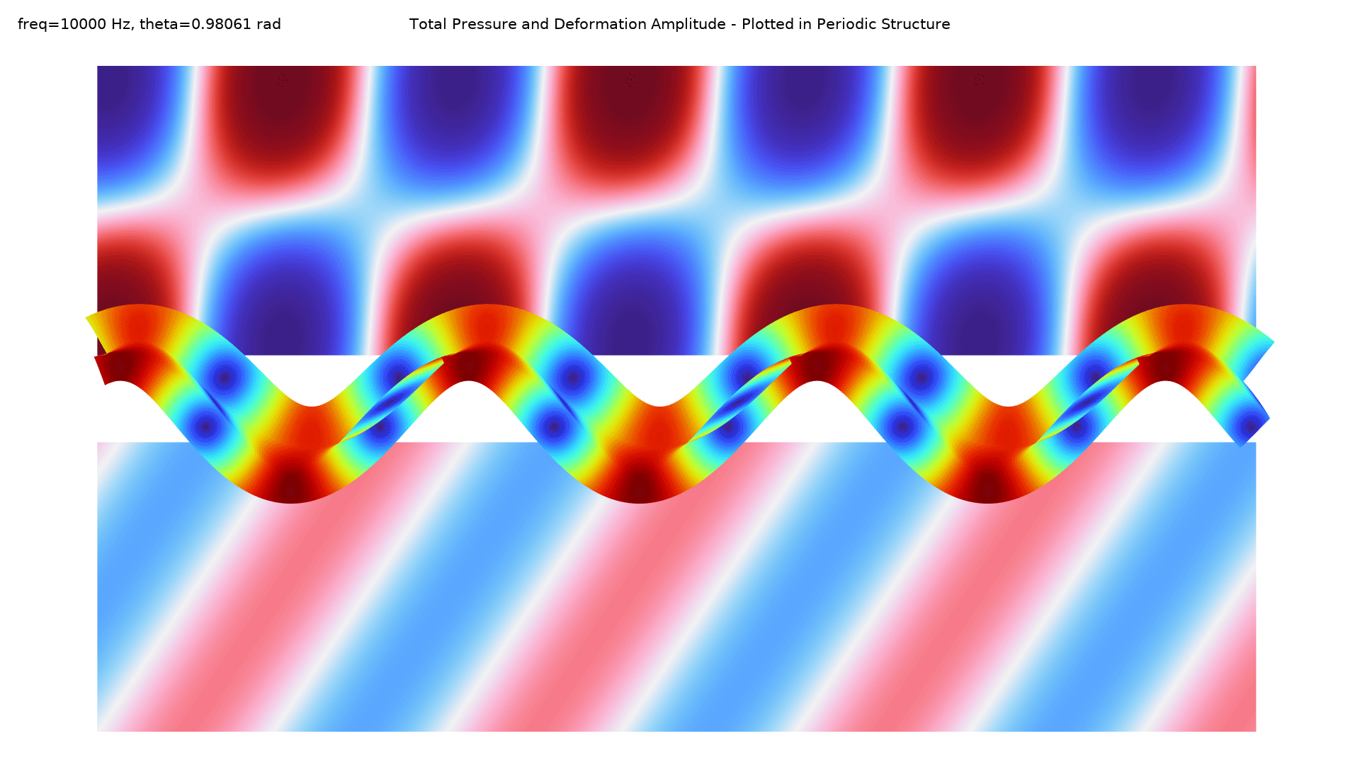
Acoustic Transmission Loss Through Multilayer Periodic Elastic Structures

The acoustic pressure response and structural deformation of a periodic multilayered system.

Download from the Application Gallery

Acoustic–Structure Interaction with Frequency Domain, Modal Solver

The response comparison between this frequency-domain model and the frequency-domain solutions.

Download from the Application Gallery